Direkt zum Inhalt

Maths2Mind Navigation

      • Terme und Zahlensysteme
      • Fest- und Gleitkommadarstellung, Zehnerpotenzen, SI-Präfixe
      • Teiler bzw Vielfache
      • Brüche und Rundungsregeln
      • Kartesische-, trigonometrische bzw. exponentielle Darstellung
      • Rechenoperationen mit komplexen Zahlen
      • Fundamentalsatz der Algebra
      • Quadratische Gleichungen mit komplexer Lösung
      • Die Schönheit der Fraktale und der Selbstähnlichkeit
      • Potenzieren
      • Wurzelziehen
      • Logarithmieren
      • Determinante
      • Matrizen
      • Lineare Gleichung mit einer Variablen
      • Quadratische Gleichung mit einer Variablen
      • Lineare Gleichungssyteme mit zwei Variablen
      • Lineare Ungleichung mit einer Variablen
      • Lineare Ungleichung mit zwei Variablen
      • Systeme linearer Ungleichungen mit einer Variablen
      • Systeme linearer Ungleichungen mit zwei Variablen
      • Quadratische Ungleichungen mit einer Variablen
      • Zahlenfolgen und Zahlenreihen
      • Modellbildung, Simulation
      • Zuordnungen
      • Eigenschaften einer Funktion
      • Lineare Funktion
      • Quadratische Funktionen (Parabel)
      • Polynomfunktionen
      • Gebrochenrationale Funktionen (Hyperbel)
      • Wurzelfunktionen
      • Potenzfunktionen
      • Exponentialfunktion
      • Logarithmusfunktion
      • Periodische Funktionen
      • Änderungsmaße
      • Differenzierbarkeit
      • Ableitungsfunktionen und Ableitungsregeln
      • Lineare Optimierung
      • Differentialgleichungen
      • Unbestimmtes Integral
      • Bestimmtes Integral
      • Stammfunktionen und Integrationsregeln
      • Numerische Integration
      • Integro-Differentialgleichungen
      • Geometrische Grundbegriffe
      • Koordinatensysteme
      • Ähnlichkeit und Kongruenz
      • Dreiecke
      • Vierecke
      • Polygone
      • Kreis, Kreissektor und Kreisbogen
      • Würfel, Quader, Prisma
      • Zylinder und Zylinderstumpf
      • Pyramide und Pyramidenstumpf
      • Kegel und Kegelstumpf
      • Kugel und Kugelkalotte
      • Winkel- und Arkusfunktionen
      • Hyperbel- und Areafunktionen
      • Vektoren
      • Vektoralgebra
      • Vektoranalysis
      • Gleichungen von Punkt, Gerade und Ebene
      • Gleichungen von Kreis, Kugel und Kegelschnitten
      • Kombinatorik
      • Beschreibende Statistik - Lagemaße
      • Beschreibende Statistik - Streumaße
      • Schließende Statistik - Wahrscheinlichkeitsrechnung
      • Explorative Statistik - Data Mining
      • Aussagen
      • Mengen
      • Prüfungsteil A - Analysis
      • Prüfungsteil A - Stochastik
      • Prüfungsteil A - Geometrie
      • Prüfungsteil B - Analysis
      • Prüfungsteil B - Stochastik
      • Prüfungsteil B - Geometrie
      • Typ 1 - Algebra und Geometrie
      • Typ 1 - Analysis
      • Typ 1 - Funktionale Abhängigkeiten
      • Typ 1 - Wahrscheinlichkeit und Statistik
      • Typ 2 - Vernetzung der Grundkompetenzen
      • Teil A Aufgaben für alle Cluster
      • Teil B Aufgaben für spezielle Cluster
      • Zins- und Zinseszinsrechnung
      • Prozent- und Promillerechnung
      • Rentenrechnung
      • Kosten- und Preistheorie
      • Investitionsrechnung
      • Künstliche Intelligenz
      • GeoGebra
      • Berechnung von Gleichstromkreisen
      • Berechnung von Wechselstromkreisen
      • Berechnung von Drehstromsystemen
      • Elektromagnetische Felder
      • Komponenten elektrischer Energienetze
      • Fourier Analyse
      • Basiseinheiten der Physik und die Naturkonstanten
      • Mechanik
      • Thermodynamik
      • Relativitätstheorien
      • Atom- und Kernphysik
      • Strahlen- und Wellentheorie des Lichtes
      • Vom Photon zum Photo
      • Photovoltaik
      • Quantenphysik
      • Standardmodell der Kosmologie
      • Standardmodell der Elementarteilchen
      • Die 4 Wechselwirkungen und der Higgs Mechanismus
      • Recruiting & Branding
      • Zusammenarbeit mit LehrerInnen und Dozenten
      • Angeleitetes autonomes Lernen
      • Testbilder
      • Taxonomie
Maths2Mind

Social Media

User account menu

  • Anmelden
Kritik, Lob, Wünsche oder Verbesserungsvorschläge?
Nehmt Euch kurz Zeit, klickt hier und schreibt an
feedback@maths2mind.com
Deine Meinung ist uns wichtig!
/contact?edit%5Bsubject%5D%5Bwidget%5D%5B0%5D%5Bvalue%5D=Nutzerfeedback

Pfadnavigation

  1. Maths2Mind
  2. Analysis
  3. Funktionen und Modelle

Funktionen und Modelle

Hier findest du folgende Inhalte

22
Formeln
16
Aufgaben
    Formeln
    Wissenspfad
    Aufgaben

    Darstellung von Funktionen

    Unter einer Funktion versteht man die eindeutige Zuordnung von jedem Element x der Definitionsmenge zu genau einem Element y der Wertemenge. Unter einer reellen Funktion versteht man die Abbildung von reellen Zahlen der Definitionsmenge auf reelle Zahlen der Wertemenge.

    \(f:{D_f} \to {W_f}\,\,\,{\text{mit}}\,\,\,x \in {D_f}\,\,\,{\text{und}}\,\,\,y \in {W_f}\)

    Es gibt mehrere gängige Schreibweisen für Funktionsgleichungen
    \(f:x \to 2{x^3}\)
    \(f\left( x \right) = 2{x^3}\)
    \(y = 2{x^3}\)


    Funktionsgleichung

    Unter einer Funktionsgleichung versteht man eine mathematische Vorschrift, die angibt, wie man aus einem gegebenen x-Wert den zugehörigen y-Wert errechnet. Dabei ist y abhängig davon, welchen Wert x man in die Funktionsgleichung einsetzt. Die Funktionsgleichung stellt die Abbildung der Werte aus der Definitionsmenge Df auf die Wertemenge Wf in Form einer Gleichung dar.

    \(f:{\Bbb R} \to {\Bbb R};\,\,\,y = f\left( x \right)\)

    Daher nennt man

    • y die abhängige Variable bzw. den Funktionswert
    • x die unabhängige Variable bzw. das Funktionsargument

    Typen wichtiger Funktionsgleichungen

    Konstante Funktion \(f\left( x \right) = c\)
    Direkt proportionale Funktion
    sie sind für d=0 eine Untermenge der linearen Funktionen
    \(f\left( x \right) = k \cdot x\)
    Lineare Funktion \(f\left( x \right) = k \cdot x + d\)
    Quadratische Funktion (Parabel) \(f\left( x \right) = a \cdot {x^2} + b \cdot x + c\)
    Indirekt proportionale Funktion (Hyperbel)
    sie sind für negative n eine Untermenge der Potenzfunktionen
    \(f\left( x \right) = \dfrac{c}{{{x^n}}} = c \cdot {x^{ - n}}\)
    Potenzfunktion \(f\left( x \right) = c \cdot {x^n}\)
    Wurzelfunktion \(f\left( x \right) = \root n \of x = {x^{\dfrac{1}{n}}}\)
    Exponentialfunktion \(\begin{array}{l} f\left( x \right) = c \cdot {a^x}\\ f\left( x \right) = c \cdot {e^x} \end{array}\)
    Logarithmusfunktion \(f\left( x \right) = {}^a\log x\)
    Periodische Funktion \(f\left( {x + T} \right) = f\left( x \right)\)
    Polynomfunktion \(f\left( x \right) = {a_n} \cdot {x^n} + {a_{n - 1}} \cdot {x^{n - 1}} + ... + {a_1} \cdot x + {a_0}\)
    uvm.

    Graph einer Funktion

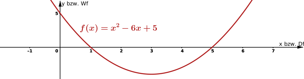
    Jedem Wert auf der x-Achse wird über die Funktion ein Punkt auf der y-Achse zugeordnet. Die Menge aller Punkte einer Funktion f(x) mit den Koordinaten (x|y=f(x)) bilden eine Kurve in der Gaus`schen Ebene, den sogenannten Graphen der Funktion.

    \(y = f\left( x \right)\)

    Geometrische Darstellung: Trägt man die unabhängige Variable x auf der x-Achse und die abhängige Variable y=f(x) auf der y-Achse auf, erhält man den Graph als eine grafische Darstellung der Funktion in Form einer Kurve.

    Funktion f f(x) = 0.5(x - 1)³ + 0.5(x - 1)² - (x - 1) $${\text{y = f(x) = 0}}{\text{.5(x - 1}}{{\text{)}}^3} + 0.5{\left( {x - 1} \right)^2} - \left( {x - 1} \right)$$ Text1 = “$${\text{y = f(x) = 0}}{\text{.5(x - 1}}{{\text{)}}^3} + 0.5{\left( {x - 1} \right)^2} - \left( {x - 1} \right)$$” $${\text{y = f(x) = 0}}{\text{.5(x - 1}}{{\text{)}}^3} + 0.5{\left( {x - 1} \right)^2} - \left( {x - 1} \right)$$ Text1 = “$${\text{y = f(x) = 0}}{\text{.5(x - 1}}{{\text{)}}^3} + 0.5{\left( {x - 1} \right)^2} - \left( {x - 1} \right)$$” $${\text{y = f(x) = 0}}{\text{.5(x - 1}}{{\text{)}}^3} + 0.5{\left( {x - 1} \right)^2} - \left( {x - 1} \right)$$ Text1 = “$${\text{y = f(x) = 0}}{\text{.5(x - 1}}{{\text{)}}^3} + 0.5{\left( {x - 1} \right)^2} - \left( {x - 1} \right)$$” $${\text{y = f(x) = 0}}{\text{.5(x - 1}}{{\text{)}}^3} + 0.5{\left( {x - 1} \right)^2} - \left( {x - 1} \right)$$ Text1 = “$${\text{y = f(x) = 0}}{\text{.5(x - 1}}{{\text{)}}^3} + 0.5{\left( {x - 1} \right)^2} - \left( {x - 1} \right)$$” $${\text{y = f(x) = 0}}{\text{.5(x - 1}}{{\text{)}}^3} + 0.5{\left( {x - 1} \right)^2} - \left( {x - 1} \right)$$ Text1 = “$${\text{y = f(x) = 0}}{\text{.5(x - 1}}{{\text{)}}^3} + 0.5{\left( {x - 1} \right)^2} - \left( {x - 1} \right)$$” $${\text{y = f(x) = 0}}{\text{.5(x - 1}}{{\text{)}}^3} + 0.5{\left( {x - 1} \right)^2} - \left( {x - 1} \right)$$ Text1 = “$${\text{y = f(x) = 0}}{\text{.5(x - 1}}{{\text{)}}^3} + 0.5{\left( {x - 1} \right)^2} - \left( {x - 1} \right)$$” $${\text{y = f(x) = 0}}{\text{.5(x - 1}}{{\text{)}}^3} + 0.5{\left( {x - 1} \right)^2} - \left( {x - 1} \right)$$ Text1 = “$${\text{y = f(x) = 0}}{\text{.5(x - 1}}{{\text{)}}^3} + 0.5{\left( {x - 1} \right)^2} - \left( {x - 1} \right)$$” $${\text{y = f(x) = 0}}{\text{.5(x - 1}}{{\text{)}}^3} + 0.5{\left( {x - 1} \right)^2} - \left( {x - 1} \right)$$ Text1 = “$${\text{y = f(x) = 0}}{\text{.5(x - 1}}{{\text{)}}^3} + 0.5{\left( {x - 1} \right)^2} - \left( {x - 1} \right)$$” $${\text{y = f(x) = 0}}{\text{.5(x - 1}}{{\text{)}}^3} + 0.5{\left( {x - 1} \right)^2} - \left( {x - 1} \right)$$ Text1 = “$${\text{y = f(x) = 0}}{\text{.5(x - 1}}{{\text{)}}^3} + 0.5{\left( {x - 1} \right)^2} - \left( {x - 1} \right)$$” $${\text{y = f(x) = 0}}{\text{.5(x - 1}}{{\text{)}}^3} + 0.5{\left( {x - 1} \right)^2} - \left( {x - 1} \right)$$ Text1 = “$${\text{y = f(x) = 0}}{\text{.5(x - 1}}{{\text{)}}^3} + 0.5{\left( {x - 1} \right)^2} - \left( {x - 1} \right)$$” $${\text{y = f(x) = 0}}{\text{.5(x - 1}}{{\text{)}}^3} + 0.5{\left( {x - 1} \right)^2} - \left( {x - 1} \right)$$ Text1 = “$${\text{y = f(x) = 0}}{\text{.5(x - 1}}{{\text{)}}^3} + 0.5{\left( {x - 1} \right)^2} - \left( {x - 1} \right)$$” $${\text{y = f(x) = 0}}{\text{.5(x - 1}}{{\text{)}}^3} + 0.5{\left( {x - 1} \right)^2} - \left( {x - 1} \right)$$ Text1 = “$${\text{y = f(x) = 0}}{\text{.5(x - 1}}{{\text{)}}^3} + 0.5{\left( {x - 1} \right)^2} - \left( {x - 1} \right)$$” $${\text{y = f(x) = 0}}{\text{.5(x - 1}}{{\text{)}}^3} + 0.5{\left( {x - 1} \right)^2} - \left( {x - 1} \right)$$ Text1 = “$${\text{y = f(x) = 0}}{\text{.5(x - 1}}{{\text{)}}^3} + 0.5{\left( {x - 1} \right)^2} - \left( {x - 1} \right)$$” $${\text{y = f(x) = 0}}{\text{.5(x - 1}}{{\text{)}}^3} + 0.5{\left( {x - 1} \right)^2} - \left( {x - 1} \right)$$ Text1 = “$${\text{y = f(x) = 0}}{\text{.5(x - 1}}{{\text{)}}^3} + 0.5{\left( {x - 1} \right)^2} - \left( {x - 1} \right)$$” $${\text{y = f(x) = 0}}{\text{.5(x - 1}}{{\text{)}}^3} + 0.5{\left( {x - 1} \right)^2} - \left( {x - 1} \right)$$ Text1 = “$${\text{y = f(x) = 0}}{\text{.5(x - 1}}{{\text{)}}^3} + 0.5{\left( {x - 1} \right)^2} - \left( {x - 1} \right)$$” $${\text{y = f(x) = 0}}{\text{.5(x - 1}}{{\text{)}}^3} + 0.5{\left( {x - 1} \right)^2} - \left( {x - 1} \right)$$ Text1 = “$${\text{y = f(x) = 0}}{\text{.5(x - 1}}{{\text{)}}^3} + 0.5{\left( {x - 1} \right)^2} - \left( {x - 1} \right)$$” $${\text{y = f(x) = 0}}{\text{.5(x - 1}}{{\text{)}}^3} + 0.5{\left( {x - 1} \right)^2} - \left( {x - 1} \right)$$ Text1 = “$${\text{y = f(x) = 0}}{\text{.5(x - 1}}{{\text{)}}^3} + 0.5{\left( {x - 1} \right)^2} - \left( {x - 1} \right)$$” $${\text{y = f(x) = 0}}{\text{.5(x - 1}}{{\text{)}}^3} + 0.5{\left( {x - 1} \right)^2} - \left( {x - 1} \right)$$ Text1 = “$${\text{y = f(x) = 0}}{\text{.5(x - 1}}{{\text{)}}^3} + 0.5{\left( {x - 1} \right)^2} - \left( {x - 1} \right)$$” $${\text{y = f(x) = 0}}{\text{.5(x - 1}}{{\text{)}}^3} + 0.5{\left( {x - 1} \right)^2} - \left( {x - 1} \right)$$ Text1 = “$${\text{y = f(x) = 0}}{\text{.5(x - 1}}{{\text{)}}^3} + 0.5{\left( {x - 1} \right)^2} - \left( {x - 1} \right)$$” $${\text{y = f(x) = 0}}{\text{.5(x - 1}}{{\text{)}}^3} + 0.5{\left( {x - 1} \right)^2} - \left( {x - 1} \right)$$ Text1 = “$${\text{y = f(x) = 0}}{\text{.5(x - 1}}{{\text{)}}^3} + 0.5{\left( {x - 1} \right)^2} - \left( {x - 1} \right)$$” $${\text{y = f(x) = 0}}{\text{.5(x - 1}}{{\text{)}}^3} + 0.5{\left( {x - 1} \right)^2} - \left( {x - 1} \right)$$ Text1 = “$${\text{y = f(x) = 0}}{\text{.5(x - 1}}{{\text{)}}^3} + 0.5{\left( {x - 1} \right)^2} - \left( {x - 1} \right)$$” $${\text{y = f(x) = 0}}{\text{.5(x - 1}}{{\text{)}}^3} + 0.5{\left( {x - 1} \right)^2} - \left( {x - 1} \right)$$ Text1 = “$${\text{y = f(x) = 0}}{\text{.5(x - 1}}{{\text{)}}^3} + 0.5{\left( {x - 1} \right)^2} - \left( {x - 1} \right)$$” $${\text{y = f(x) = 0}}{\text{.5(x - 1}}{{\text{)}}^3} + 0.5{\left( {x - 1} \right)^2} - \left( {x - 1} \right)$$ Text1 = “$${\text{y = f(x) = 0}}{\text{.5(x - 1}}{{\text{)}}^3} + 0.5{\left( {x - 1} \right)^2} - \left( {x - 1} \right)$$” $${\text{y = f(x) = 0}}{\text{.5(x - 1}}{{\text{)}}^3} + 0.5{\left( {x - 1} \right)^2} - \left( {x - 1} \right)$$ Text1 = “$${\text{y = f(x) = 0}}{\text{.5(x - 1}}{{\text{)}}^3} + 0.5{\left( {x - 1} \right)^2} - \left( {x - 1} \right)$$” $${\text{y = f(x) = 0}}{\text{.5(x - 1}}{{\text{)}}^3} + 0.5{\left( {x - 1} \right)^2} - \left( {x - 1} \right)$$ Text1 = “$${\text{y = f(x) = 0}}{\text{.5(x - 1}}{{\text{)}}^3} + 0.5{\left( {x - 1} \right)^2} - \left( {x - 1} \right)$$” $${\text{y = f(x) = 0}}{\text{.5(x - 1}}{{\text{)}}^3} + 0.5{\left( {x - 1} \right)^2} - \left( {x - 1} \right)$$ Text1 = “$${\text{y = f(x) = 0}}{\text{.5(x - 1}}{{\text{)}}^3} + 0.5{\left( {x - 1} \right)^2} - \left( {x - 1} \right)$$” $${\text{y = f(x) = 0}}{\text{.5(x - 1}}{{\text{)}}^3} + 0.5{\left( {x - 1} \right)^2} - \left( {x - 1} \right)$$ Text1 = “$${\text{y = f(x) = 0}}{\text{.5(x - 1}}{{\text{)}}^3} + 0.5{\left( {x - 1} \right)^2} - \left( {x - 1} \right)$$” $${\text{y = f(x) = 0}}{\text{.5(x - 1}}{{\text{)}}^3} + 0.5{\left( {x - 1} \right)^2} - \left( {x - 1} \right)$$ Text1 = “$${\text{y = f(x) = 0}}{\text{.5(x - 1}}{{\text{)}}^3} + 0.5{\left( {x - 1} \right)^2} - \left( {x - 1} \right)$$” $${\text{y = f(x) = 0}}{\text{.5(x - 1}}{{\text{)}}^3} + 0.5{\left( {x - 1} \right)^2} - \left( {x - 1} \right)$$ Text1 = “$${\text{y = f(x) = 0}}{\text{.5(x - 1}}{{\text{)}}^3} + 0.5{\left( {x - 1} \right)^2} - \left( {x - 1} \right)$$” $${\text{y = f(x) = 0}}{\text{.5(x - 1}}{{\text{)}}^3} + 0.5{\left( {x - 1} \right)^2} - \left( {x - 1} \right)$$ Text1 = “$${\text{y = f(x) = 0}}{\text{.5(x - 1}}{{\text{)}}^3} + 0.5{\left( {x - 1} \right)^2} - \left( {x - 1} \right)$$” $${\text{y = f(x) = 0}}{\text{.5(x - 1}}{{\text{)}}^3} + 0.5{\left( {x - 1} \right)^2} - \left( {x - 1} \right)$$ Text1 = “$${\text{y = f(x) = 0}}{\text{.5(x - 1}}{{\text{)}}^3} + 0.5{\left( {x - 1} \right)^2} - \left( {x - 1} \right)$$” $${\text{y = f(x) = 0}}{\text{.5(x - 1}}{{\text{)}}^3} + 0.5{\left( {x - 1} \right)^2} - \left( {x - 1} \right)$$ Text1 = “$${\text{y = f(x) = 0}}{\text{.5(x - 1}}{{\text{)}}^3} + 0.5{\left( {x - 1} \right)^2} - \left( {x - 1} \right)$$”


    Wertetabelle einer Funktion

    Trägt man in einer 2-spaltigen Tabelle in der 1. Spalte die x-Werte gemäß der Definitionsmenge Df ein und in der 2. Spalte die y=f(x) Werte gemäß der Wertemenge Wf, so erhält man Zahlenpaare, die die Zeilen der Wertetabelle bilden.

    x y=f(x)
    x1 f(x1)
    x2 f(x2)
    ... ...
    xi f(xi)

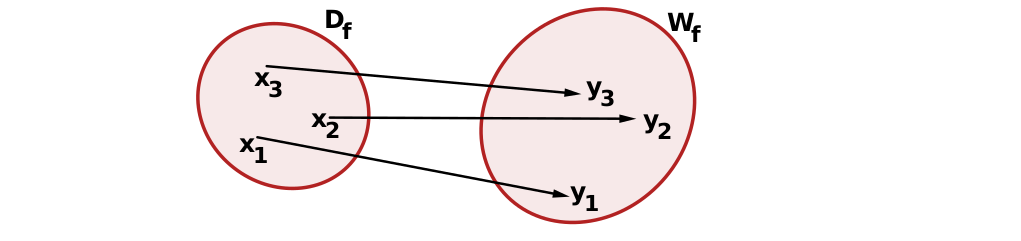
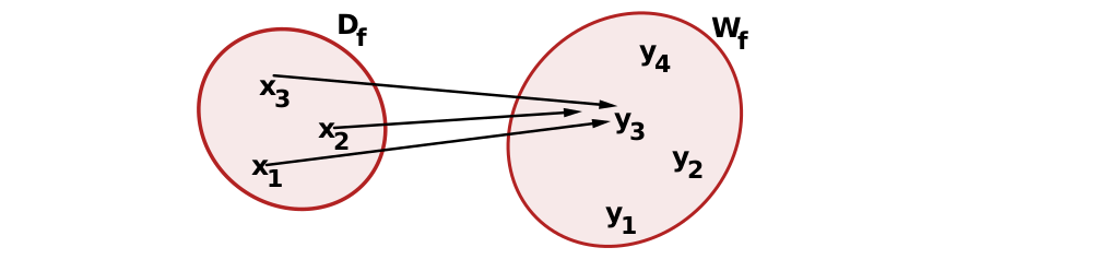
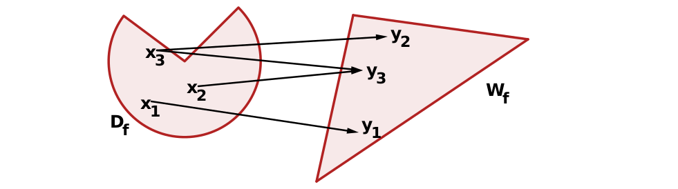
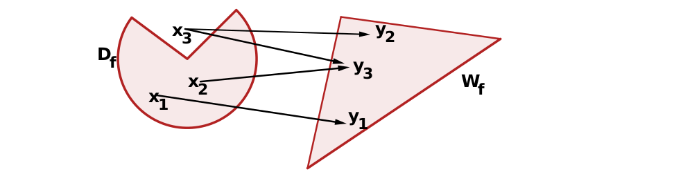
    Mengendiagramm einer Funktion

    Grafische Gegenüberstellung von Definitionsmenge und Wertemenge einer Funktion, wobei die Wertepaare durch Pfeile mit einander verbunden werden

    Ellipse D_f Ellipse D_f: Ellipse mit Brennpunkten A, B durch C Ellipse D_f Ellipse D_f: Ellipse mit Brennpunkten A, B durch C Ellipse W_f Ellipse W_f: Ellipse mit Brennpunkten D, E durch F Ellipse W_f Ellipse W_f: Ellipse mit Brennpunkten D, E durch F Vektor u Vektor u: Vektor[x_4, y_1] Vektor u Vektor u: Vektor[x_4, y_1] Vektor v Vektor v: Vektor[x_1, y_2] Vektor v Vektor v: Vektor[x_1, y_2] Vektor w Vektor w: Vektor[x_3, y_4] Vektor w Vektor w: Vektor[x_3, y_4] D_f Text1 = "D_f" D_f Text1 = "D_f" W_f Text2 = "W_f" W_f Text2 = "W_f" x_1 Text3 = "x_1" x_1 Text3 = "x_1" x_2 Text4 = "x_2" x_2 Text4 = "x_2" x_3 Text5 = "x_3" x_3 Text5 = "x_3" y_1 Text6 = "y_1" y_1 Text6 = "y_1" y_2 Text7 = "y_2" y_2 Text7 = "y_2" y_3 Text8 = "y_3" y_3 Text8 = "y_3"

    Funktion
    Definitionsbereich
    Wertebereich
    Funktionsgleichung
    abhängige Variable
    unabhängige Variable
    Konstante Funktion
    Lineare Funktion
    Quadratische Funktion
    Indirekt proportionale Funktion
    Potenzfunktionen
    Wurzelfunktionen
    Exponentialfunktionen
    Logarithmusfunktionen
    Periodische Funktion
    Polynomfunktion
    Direkt proportionale Funktion
    Funktionswerte
    Argument einer Funktion
    Funktionen Überblick
    Reelle Funktionen
    Darstellung einer Funktion
    Graph einer Funktion
    Wertetabelle einer Funktion
    Fragen oder Feedback

    Schon den nächsten Urlaub geplant?
    Auf maths2mind kostenlos auf Prüfungen vorbereiten!
    Nach der Prüfung in Ruhe entspannen

    Startseite
    rgb(244,123,130)
    Bild
    Illustration Medidation 1050x450
    Startseite
    Wissenspfad
    Aufgaben

    Polynomfunktionen n-ten Grades

    Ein Polynom ist die Summe von mehreren Potenzfunktionen. Der Grad der Polynomfunktion „n“ entspricht der höchsten vorkommenden Potenz von der Variablen x. Alle Polynomfunktionen verlaufen durch den Punkt \(P\left( {0\left| {{a_0}} \right.} \right)\). Der Definitionsbereich von Polynomfunktionen ist nicht eingeschränkt, daher gilt: \(D = {\Bbb R}\). Polynomfunktionen werden auch ganzrationale Funktionen genannt.

    \(f\left( x \right) = {a_n} \cdot {x^n} + {a_{n - 1}} \cdot {x^{n - 1}} + ... + {a_2} \cdot {x^2} + {a_1} \cdot x + {a_0}\)

    \(f\left( x \right) = \sum\limits_{i = 0}^n {{a_i} \cdot {x^i}} \)

    \(f\left( x \right) = c \cdot \left( {x - {x_1}} \right) \cdot \left( {x - {x_2}} \right) \cdot ... \cdot \left( {x - {x_n}} \right){\text{ wobei }}{{\text{x}}_n}{\text{ die n Nullstellen sind}}\)

    wobei:

    \(\eqalign{ & {a_n},{a_{n - 1}},...,{a_1},{a_0} \cr & n \in N;\,\,\,\,\,{a_i} \in {\Bbb R};\,\,\,\,\,{a_n} \ne 0 \cr} \) Koeffizienten
    ai i-ter Koeffizient
    n höchste Potenz
    \({a_2} \cdot {x^2}\) quadratisches Glied
    \({a_1} \cdot x\) lineares Glied
    \({a_0}\) konstantes Glied

    Die wichtigsten Polynomfunktionen:


    n=0:
    konstante Funktion
    \(f\left( x \right) = {a_0}\)

    • ​0 oder bei f(x)== unendlich viele Nullstellen
    • 0 Extremstellen
    • 0 Wendestellen
    • Typischer Graph verläuft parallel zur x-Achse
       

    n=1:
    lineare Funktion
    \(f\left( x \right) = {a_1} \cdot x + {a_0} = k \cdot x + d\)

    • ​1 Nullstelle
    • 0 Extremstellen
    • 0 Wendestellen
    • Typischer Graph ist eine Gerade, welche die x und die y-Achse schneidet
       

    n=2:
    quadratische Funktion bzw. Parabel
    \(f\left( x \right) = {a_2} \cdot {x^2} + {a_1} \cdot x + {a_0} = a \cdot {x^2} + b \cdot x + c\)

    • ​0, 1 oder 2 Nullstellen
    • 1 Extremstelle, bei: \(x = - \dfrac{{{a_1}}}{{2{a_2}}}{\text{ für }}{{\text{a}}_2} \ne 0\)
    • 0 Wendestelle
    • Typischer Graph ist eine Parabel
       

    Die quadratische Funktion setzt sich aus einem quadratischen, einem linearen und einem konstanten Glied zusammen.

    • a > 0 → Graph noch oben offen (U-förmig), d.h. der Scheitelpunkt der Parabel ist ein Tiefpunkt
    • a < 0 → Graph nach unten offen, d.h. der Scheitelpunkt der Parabel ist ein Hochpunkt
    • Der Faktor b bewirkt eine Schiebung in x und y-Richtung.
    • b = 0 → Der Scheitelpunkt der Parabel liegt auf der y-Achse. Wo auf der y-Achse der Scheitelpunkt liegt, hängt dann nur von c ab
    • b = 0 und c = 0 → Scheitelpunkt der Parabel liegt im Ursprung vom Koordinatensystem
    • Der Faktor c bewirkt ausschließlich eine Verschiebung noch oben (c>0) oder nach unten (c<0)

    n=3:
    kubische Funktion
    \(f(x) = {a_3} \cdot {x^3} + {a_2} \cdot {x^2} + {a_1} \cdot x + {a_0}\)

    • 1, 2 oder 3 Nullstellen
    • 0 oder 2 Extremstellen
    • 1 Wendestelle
    • Typischer Graph verläuft s-förmig
       

    n=4:
    \(f(x) = {a_4} \cdot {x^4} + {a_3} \cdot {x^3} + {a_2} \cdot {x^2} + {a_1} \cdot x + {a_0}\)

    • 0 .. 4 Nullstellen
    • 1 oder 3 Extremstellen
    • 0 oder 2 Wendestellen
    • Typischer Graph verläuft w-förmig
       

    Nullstellen: Maximale Anzahl der Nullstellen = Grad der Funktion.

    • Wenn „n“ ungerade ist, dann haben sie mindestens eine Lösung in \({\Bbb R}\)
       

    Extremstellen: Maximale Anzahl der Extremstellen = Grad der Funktion n minus 1
     

    Wendepunkte: Maximale Anzahl der Wendepunkte = Grad der Funktion n minus 2

    • \(n \geqslant 3\) und n gerade: 0, 2, 4,.. Wendestellen
    • \(n \geqslant 3\) und n ungerade: mindestens 1 Wendestelle
       

    konstantes Glied: Das konstante Glied erhält man immer an der Stelle x=0. Daher kann man es aus einem Graph auf der y-Achse (\(P\left( {0\left| {{a_n}} \right.} \right)\)) direkt ablesen.

    Polynomfunktion n-ten Grades
    Konstante Funktion
    Lineare Funktion
    Quadratische Funktion
    Anzahl an Nullstellen
    Anzahl an Extremstellen
    Anzahl an Wendestellen
    Koeffizient
    kubische Funktion
    ganzrationale Funktionen
    Verschiebung einer Parabel
    Fragen oder Feedback
    Wissenspfad

    Taylorpolynom

    Das Taylorpolynom bietet die Möglichkeit eine komplizierte Funktion f(x), an einer vorgegebenen Stelle x0 durch eine Polynomfunktion zu approximieren. Man spricht dann von einem „Taylor-Polynom n-ten Grades an der Entwicklungsstelle x0 “.

    \(\eqalign{ & f\left( x \right) \approx \cr & f\left( {{x_0}} \right) + \dfrac{{f'\left( {{x_0}} \right)}}{{1!}} \cdot \left( {x - {x_0}} \right) + \dfrac{{f''\left( {{x_0}} \right)}}{{2!}} \cdot {\left( {x - {x_0}} \right)^2} + ... + \dfrac{{{f^{\left( n \right)}}\left( {{x_0}} \right)}}{{n!}} \cdot {\left( {x - {x_0}} \right)^n} = \cr & = \sum\limits_{i = 0}^n {\dfrac{{{f^{\left( i \right)}}\left( {{x_0}} \right)}}{{i!}}} {\left( {x - {x_0}} \right)^i} \cr}\)


    Den Fehler, der bei der Näherung durch das Taylorpolynom gemacht wurde, kann man mit Hilfe der Formeln von Lagrange oder Cauchy abschätzen. Die beiden Formeln für das Restglied \({R_{n,{x_0}}}\left( x \right)\) d.h. für den Fehler des n-ten Taylorpolynoms um den Entwicklungspunkt x0 an der Stelle x lauten:

    nach Lagrange: \({R_{n,{x_0}}}\left( x \right) = \dfrac{{{f^{\left( {n + 1} \right)}}\left( c \right)}}{{\left( {n + 1} \right)!}} \cdot {\left( {x - {x_0}} \right)^{\left( {n + 1} \right)}}\,\,\,\,\,{\text{wobei}}\,\,\,c \in \left[ {{x_0},x} \right]\)


    nach Cauchy: \({R_{n,{x_0}}}\left( x \right) = \dfrac{{{f^{\left( {n + 1} \right)}}\left( c \right)}}{{n!}} \cdot {\left( {x - c} \right)^{\left( n \right)}} \cdot \left( {x - {x_0}} \right)\,\,\,\,\,{\text{wobei}}\,\,\,c \in \left[ {{x_0},x} \right]\)

    Taylorpolynom (Differenzierbarkeit)
    Fragen oder Feedback
    Wissenspfad
    Aufgaben

    Grad einer Funktion

    Audiodatei

    Polynomfunktionen, auch ganzrationale Funktionen genannt, bestehen aus einer Summe bzw. Differenz von Termen, den sogenannten Gliedern. Diese Glieder sind ihrerseits das Produkt aus einer Zahl und einer Potenz, etwa 2x². Zur besseren Lesbarkeit werden die Glieder geordnet nach der Höhe ihrer Exponenten angeschrieben. Der höchste vorkommende Exponent der Variablen, gibt zugleich den Grad der Polynomfunktion an. So handelt es sich bei 2x²+x um eine Polynomfunktion zweiten Grades.

    Aus dem Grad einer Funktion kann man Aussagen über deren Graph herleiten:

    • Eine konstante Funktion, die nicht konstant null ist, hat den Grad 0. Ihr Graph ist eine horizontale Gerade.
    • Eine lineare Funktion hat den Grad 1. Ihr Graph ist eine steigende oder fallende Gerade.
    • Eine quadratische Funktion hat den Grad 2. Ihr Graph ist eine Parabel.
    • Eine kubische Funktion hat den Grad 3. Ihr Graph weist einen s-förmigen Verlauf auf.
    • Eine Polynomfunktion vom 4. Grad kann einen w-förmigen Verlauf haben.

    Aus dem Grad einer Funktion kann man Aussagen über besondere Funktionswerte herleiten:

    • Der Grad einer Funktion ist gleich der maximalen Anzahl der Nullstellen (mit deren Vielfachheit gezählt). Vergleiche dazu den „Fundamentalsatz der Algebra“, welcher für den Bereich der komplexe Zahlen gilt.
    • Grad einer Funktion minus 1, ergibt die maximale Anzahl der Extremstellen.
    • Grad einer Funktion minus 2, ergibt die maximale Anzahl der Wendestellen.


    • Wenn der höchste Exponent der Funktion gerade ist, dann streben, wenn x gegen plus minus unendlich geht, die beiden Grenzwerte gegen Unendlich, wobei beide Grenzwerte das gleiche Vorzeichen haben.

    • Wenn der höchste Exponent der Funktion ungerade ist, dann streben, wenn x gegen plus minus unendlich geht, die beiden Grenzwerte gegen Unendlich, wobei beide Grenzwerte unterschiedliche Vorzeichen haben.


    Graphen von Funkionen unterschiedlichen Grades

    Die Beschriftung vom Graph der jeweiligen Funktion erfolgt einmal in der Polynomform und einmal in der Linearfaktordarstellung, in der man die Nullstellen der Funktion sofort ablesen kann, indem man dasjenige x bestimmt, für das der Wert der jeweiligen Klammer zu Null wird:

    Funktion vom 0. Grad: Konstante Funktion
    Funktion g g(x) = 1 f(x)=x⁰=1 Text1 = “f(x)=x⁰=1” f(x)=x⁰=1 Text1 = “f(x)=x⁰=1” f(x)=x⁰=1 Text1 = “f(x)=x⁰=1” f(x)=x⁰=1 Text1 = “f(x)=x⁰=1” f(x)=x⁰=1 Text1 = “f(x)=x⁰=1” f(x)=x⁰=1 Text1 = “f(x)=x⁰=1” f(x)=x⁰=1 Text1 = “f(x)=x⁰=1” f(x)=x⁰=1 Text1 = “f(x)=x⁰=1” f(x)=x⁰=1 Text1 = “f(x)=x⁰=1”


    Funktion vom 1. Grad: Gerade, ob sie steigt oder fällt hängt vom Parameter vor der linearen Variable ab
    Funktion g g(x) = x - 2 f(x) = x-2=(x - 2) Text1 = "f(x) = x-2=(x - 2)" f(x) = x-2=(x - 2) Text1 = "f(x) = x-2=(x - 2)" f(x) = x-2=(x - 2) Text1 = "f(x) = x-2=(x - 2)" f(x) = x-2=(x - 2) Text1 = "f(x) = x-2=(x - 2)" f(x) = x-2=(x - 2) Text1 = "f(x) = x-2=(x - 2)" f(x) = x-2=(x - 2) Text1 = "f(x) = x-2=(x - 2)" f(x) = x-2=(x - 2) Text1 = "f(x) = x-2=(x - 2)" f(x) = x-2=(x - 2) Text1 = "f(x) = x-2=(x - 2)" f(x) = x-2=(x - 2) Text1 = "f(x) = x-2=(x - 2)" f(x) = x-2=(x - 2) Text1 = "f(x) = x-2=(x - 2)" f(x) = x-2=(x - 2) Text1 = "f(x) = x-2=(x - 2)" f(x) = x-2=(x - 2) Text1 = "f(x) = x-2=(x - 2)" f(x) = x-2=(x - 2) Text1 = "f(x) = x-2=(x - 2)" f(x) = x-2=(x - 2) Text1 = "f(x) = x-2=(x - 2)"


    Funktion vom 2. Grad: Parabel
    Funktion f f(x) = (x - 0.8) (x - 2.25) f(x)={x^2} - 3,05 \cdot x + 1,8 = (x - 0,8) \cdot (x - 2,25) Text1 = "f(x)={x^2} - 3,05 \cdot x + 1,8 = (x - 0,8) \cdot (x - 2,25)" f(x)={x^2} - 3,05 \cdot x + 1,8 = (x - 0,8) \cdot (x - 2,25) Text1 = "f(x)={x^2} - 3,05 \cdot x + 1,8 = (x - 0,8) \cdot (x - 2,25)" f(x)={x^2} - 3,05 \cdot x + 1,8 = (x - 0,8) \cdot (x - 2,25) Text1 = "f(x)={x^2} - 3,05 \cdot x + 1,8 = (x - 0,8) \cdot (x - 2,25)" f(x)={x^2} - 3,05 \cdot x + 1,8 = (x - 0,8) \cdot (x - 2,25) Text1 = "f(x)={x^2} - 3,05 \cdot x + 1,8 = (x - 0,8) \cdot (x - 2,25)" f(x)={x^2} - 3,05 \cdot x + 1,8 = (x - 0,8) \cdot (x - 2,25) Text1 = "f(x)={x^2} - 3,05 \cdot x + 1,8 = (x - 0,8) \cdot (x - 2,25)" f(x)={x^2} - 3,05 \cdot x + 1,8 = (x - 0,8) \cdot (x - 2,25) Text1 = "f(x)={x^2} - 3,05 \cdot x + 1,8 = (x - 0,8) \cdot (x - 2,25)" f(x)={x^2} - 3,05 \cdot x + 1,8 = (x - 0,8) \cdot (x - 2,25) Text1 = "f(x)={x^2} - 3,05 \cdot x + 1,8 = (x - 0,8) \cdot (x - 2,25)" f(x)={x^2} - 3,05 \cdot x + 1,8 = (x - 0,8) \cdot (x - 2,25) Text1 = "f(x)={x^2} - 3,05 \cdot x + 1,8 = (x - 0,8) \cdot (x - 2,25)" f(x)={x^2} - 3,05 \cdot x + 1,8 = (x - 0,8) \cdot (x - 2,25) Text1 = "f(x)={x^2} - 3,05 \cdot x + 1,8 = (x - 0,8) \cdot (x - 2,25)" f(x)={x^2} - 3,05 \cdot x + 1,8 = (x - 0,8) \cdot (x - 2,25) Text1 = "f(x)={x^2} - 3,05 \cdot x + 1,8 = (x - 0,8) \cdot (x - 2,25)" f(x)={x^2} - 3,05 \cdot x + 1,8 = (x - 0,8) \cdot (x - 2,25) Text1 = "f(x)={x^2} - 3,05 \cdot x + 1,8 = (x - 0,8) \cdot (x - 2,25)" f(x)={x^2} - 3,05 \cdot x + 1,8 = (x - 0,8) \cdot (x - 2,25) Text1 = "f(x)={x^2} - 3,05 \cdot x + 1,8 = (x - 0,8) \cdot (x - 2,25)" f(x)={x^2} - 3,05 \cdot x + 1,8 = (x - 0,8) \cdot (x - 2,25) Text1 = "f(x)={x^2} - 3,05 \cdot x + 1,8 = (x - 0,8) \cdot (x - 2,25)" f(x)={x^2} - 3,05 \cdot x + 1,8 = (x - 0,8) \cdot (x - 2,25) Text1 = "f(x)={x^2} - 3,05 \cdot x + 1,8 = (x - 0,8) \cdot (x - 2,25)" f(x)={x^2} - 3,05 \cdot x + 1,8 = (x - 0,8) \cdot (x - 2,25) Text1 = "f(x)={x^2} - 3,05 \cdot x + 1,8 = (x - 0,8) \cdot (x - 2,25)" f(x)={x^2} - 3,05 \cdot x + 1,8 = (x - 0,8) \cdot (x - 2,25) Text1 = "f(x)={x^2} - 3,05 \cdot x + 1,8 = (x - 0,8) \cdot (x - 2,25)" f(x)={x^2} - 3,05 \cdot x + 1,8 = (x - 0,8) \cdot (x - 2,25) Text1 = "f(x)={x^2} - 3,05 \cdot x + 1,8 = (x - 0,8) \cdot (x - 2,25)" f(x)={x^2} - 3,05 \cdot x + 1,8 = (x - 0,8) \cdot (x - 2,25) Text1 = "f(x)={x^2} - 3,05 \cdot x + 1,8 = (x - 0,8) \cdot (x - 2,25)" f(x)={x^2} - 3,05 \cdot x + 1,8 = (x - 0,8) \cdot (x - 2,25) Text1 = "f(x)={x^2} - 3,05 \cdot x + 1,8 = (x - 0,8) \cdot (x - 2,25)" f(x)={x^2} - 3,05 \cdot x + 1,8 = (x - 0,8) \cdot (x - 2,25) Text1 = "f(x)={x^2} - 3,05 \cdot x + 1,8 = (x - 0,8) \cdot (x - 2,25)" f(x)={x^2} - 3,05 \cdot x + 1,8 = (x - 0,8) \cdot (x - 2,25) Text1 = "f(x)={x^2} - 3,05 \cdot x + 1,8 = (x - 0,8) \cdot (x - 2,25)" f(x)={x^2} - 3,05 \cdot x + 1,8 = (x - 0,8) \cdot (x - 2,25) Text1 = "f(x)={x^2} - 3,05 \cdot x + 1,8 = (x - 0,8) \cdot (x - 2,25)" f(x)={x^2} - 3,05 \cdot x + 1,8 = (x - 0,8) \cdot (x - 2,25) Text1 = "f(x)={x^2} - 3,05 \cdot x + 1,8 = (x - 0,8) \cdot (x - 2,25)" f(x)={x^2} - 3,05 \cdot x + 1,8 = (x - 0,8) \cdot (x - 2,25) Text1 = "f(x)={x^2} - 3,05 \cdot x + 1,8 = (x - 0,8) \cdot (x - 2,25)" f(x)={x^2} - 3,05 \cdot x + 1,8 = (x - 0,8) \cdot (x - 2,25) Text1 = "f(x)={x^2} - 3,05 \cdot x + 1,8 = (x - 0,8) \cdot (x - 2,25)" f(x)={x^2} - 3,05 \cdot x + 1,8 = (x - 0,8) \cdot (x - 2,25) Text1 = "f(x)={x^2} - 3,05 \cdot x + 1,8 = (x - 0,8) \cdot (x - 2,25)" f(x)={x^2} - 3,05 \cdot x + 1,8 = (x - 0,8) \cdot (x - 2,25) Text1 = "f(x)={x^2} - 3,05 \cdot x + 1,8 = (x - 0,8) \cdot (x - 2,25)" f(x)={x^2} - 3,05 \cdot x + 1,8 = (x - 0,8) \cdot (x - 2,25) Text1 = "f(x)={x^2} - 3,05 \cdot x + 1,8 = (x - 0,8) \cdot (x - 2,25)" f(x)={x^2} - 3,05 \cdot x + 1,8 = (x - 0,8) \cdot (x - 2,25) Text1 = "f(x)={x^2} - 3,05 \cdot x + 1,8 = (x - 0,8) \cdot (x - 2,25)" f(x)={x^2} - 3,05 \cdot x + 1,8 = (x - 0,8) \cdot (x - 2,25) Text1 = "f(x)={x^2} - 3,05 \cdot x + 1,8 = (x - 0,8) \cdot (x - 2,25)" f(x)={x^2} - 3,05 \cdot x + 1,8 = (x - 0,8) \cdot (x - 2,25) Text1 = "f(x)={x^2} - 3,05 \cdot x + 1,8 = (x - 0,8) \cdot (x - 2,25)" f(x)={x^2} - 3,05 \cdot x + 1,8 = (x - 0,8) \cdot (x - 2,25) Text1 = "f(x)={x^2} - 3,05 \cdot x + 1,8 = (x - 0,8) \cdot (x - 2,25)" f(x)={x^2} - 3,05 \cdot x + 1,8 = (x - 0,8) \cdot (x - 2,25) Text1 = "f(x)={x^2} - 3,05 \cdot x + 1,8 = (x - 0,8) \cdot (x - 2,25)" f(x)={x^2} - 3,05 \cdot x + 1,8 = (x - 0,8) \cdot (x - 2,25) Text1 = "f(x)={x^2} - 3,05 \cdot x + 1,8 = (x - 0,8) \cdot (x - 2,25)" f(x)={x^2} - 3,05 \cdot x + 1,8 = (x - 0,8) \cdot (x - 2,25) Text1 = "f(x)={x^2} - 3,05 \cdot x + 1,8 = (x - 0,8) \cdot (x - 2,25)"


    Funktion vom 3. Grad: S-förmiger Kurvenverlauf von links unten nach rechts oben
    Funktion g g(x) = (x + 1) (x + 2) (x - 1) f\left( x \right) = {x^3} + 2{x^2} - x - 2 = (x + 1) \cdot \left( {x + 2} \right) \cdot \left( {x - 1} \right) Text1 = "f\left( x \right) = {x^3} + 2{x^2} - x - 2 = (x + 1) \cdot \left( {x + 2} \right) \cdot \left( {x - 1} \right)" f\left( x \right) = {x^3} + 2{x^2} - x - 2 = (x + 1) \cdot \left( {x + 2} \right) \cdot \left( {x - 1} \right) Text1 = "f\left( x \right) = {x^3} + 2{x^2} - x - 2 = (x + 1) \cdot \left( {x + 2} \right) \cdot \left( {x - 1} \right)" f\left( x \right) = {x^3} + 2{x^2} - x - 2 = (x + 1) \cdot \left( {x + 2} \right) \cdot \left( {x - 1} \right) Text1 = "f\left( x \right) = {x^3} + 2{x^2} - x - 2 = (x + 1) \cdot \left( {x + 2} \right) \cdot \left( {x - 1} \right)" f\left( x \right) = {x^3} + 2{x^2} - x - 2 = (x + 1) \cdot \left( {x + 2} \right) \cdot \left( {x - 1} \right) Text1 = "f\left( x \right) = {x^3} + 2{x^2} - x - 2 = (x + 1) \cdot \left( {x + 2} \right) \cdot \left( {x - 1} \right)" f\left( x \right) = {x^3} + 2{x^2} - x - 2 = (x + 1) \cdot \left( {x + 2} \right) \cdot \left( {x - 1} \right) Text1 = "f\left( x \right) = {x^3} + 2{x^2} - x - 2 = (x + 1) \cdot \left( {x + 2} \right) \cdot \left( {x - 1} \right)" f\left( x \right) = {x^3} + 2{x^2} - x - 2 = (x + 1) \cdot \left( {x + 2} \right) \cdot \left( {x - 1} \right) Text1 = "f\left( x \right) = {x^3} + 2{x^2} - x - 2 = (x + 1) \cdot \left( {x + 2} \right) \cdot \left( {x - 1} \right)" f\left( x \right) = {x^3} + 2{x^2} - x - 2 = (x + 1) \cdot \left( {x + 2} \right) \cdot \left( {x - 1} \right) Text1 = "f\left( x \right) = {x^3} + 2{x^2} - x - 2 = (x + 1) \cdot \left( {x + 2} \right) \cdot \left( {x - 1} \right)" f\left( x \right) = {x^3} + 2{x^2} - x - 2 = (x + 1) \cdot \left( {x + 2} \right) \cdot \left( {x - 1} \right) Text1 = "f\left( x \right) = {x^3} + 2{x^2} - x - 2 = (x + 1) \cdot \left( {x + 2} \right) \cdot \left( {x - 1} \right)" f\left( x \right) = {x^3} + 2{x^2} - x - 2 = (x + 1) \cdot \left( {x + 2} \right) \cdot \left( {x - 1} \right) Text1 = "f\left( x \right) = {x^3} + 2{x^2} - x - 2 = (x + 1) \cdot \left( {x + 2} \right) \cdot \left( {x - 1} \right)" f\left( x \right) = {x^3} + 2{x^2} - x - 2 = (x + 1) \cdot \left( {x + 2} \right) \cdot \left( {x - 1} \right) Text1 = "f\left( x \right) = {x^3} + 2{x^2} - x - 2 = (x + 1) \cdot \left( {x + 2} \right) \cdot \left( {x - 1} \right)" f\left( x \right) = {x^3} + 2{x^2} - x - 2 = (x + 1) \cdot \left( {x + 2} \right) \cdot \left( {x - 1} \right) Text1 = "f\left( x \right) = {x^3} + 2{x^2} - x - 2 = (x + 1) \cdot \left( {x + 2} \right) \cdot \left( {x - 1} \right)" f\left( x \right) = {x^3} + 2{x^2} - x - 2 = (x + 1) \cdot \left( {x + 2} \right) \cdot \left( {x - 1} \right) Text1 = "f\left( x \right) = {x^3} + 2{x^2} - x - 2 = (x + 1) \cdot \left( {x + 2} \right) \cdot \left( {x - 1} \right)" f\left( x \right) = {x^3} + 2{x^2} - x - 2 = (x + 1) \cdot \left( {x + 2} \right) \cdot \left( {x - 1} \right) Text1 = "f\left( x \right) = {x^3} + 2{x^2} - x - 2 = (x + 1) \cdot \left( {x + 2} \right) \cdot \left( {x - 1} \right)" f\left( x \right) = {x^3} + 2{x^2} - x - 2 = (x + 1) \cdot \left( {x + 2} \right) \cdot \left( {x - 1} \right) Text1 = "f\left( x \right) = {x^3} + 2{x^2} - x - 2 = (x + 1) \cdot \left( {x + 2} \right) \cdot \left( {x - 1} \right)" f\left( x \right) = {x^3} + 2{x^2} - x - 2 = (x + 1) \cdot \left( {x + 2} \right) \cdot \left( {x - 1} \right) Text1 = "f\left( x \right) = {x^3} + 2{x^2} - x - 2 = (x + 1) \cdot \left( {x + 2} \right) \cdot \left( {x - 1} \right)" f\left( x \right) = {x^3} + 2{x^2} - x - 2 = (x + 1) \cdot \left( {x + 2} \right) \cdot \left( {x - 1} \right) Text1 = "f\left( x \right) = {x^3} + 2{x^2} - x - 2 = (x + 1) \cdot \left( {x + 2} \right) \cdot \left( {x - 1} \right)" f\left( x \right) = {x^3} + 2{x^2} - x - 2 = (x + 1) \cdot \left( {x + 2} \right) \cdot \left( {x - 1} \right) Text1 = "f\left( x \right) = {x^3} + 2{x^2} - x - 2 = (x + 1) \cdot \left( {x + 2} \right) \cdot \left( {x - 1} \right)" f\left( x \right) = {x^3} + 2{x^2} - x - 2 = (x + 1) \cdot \left( {x + 2} \right) \cdot \left( {x - 1} \right) Text1 = "f\left( x \right) = {x^3} + 2{x^2} - x - 2 = (x + 1) \cdot \left( {x + 2} \right) \cdot \left( {x - 1} \right)" f\left( x \right) = {x^3} + 2{x^2} - x - 2 = (x + 1) \cdot \left( {x + 2} \right) \cdot \left( {x - 1} \right) Text1 = "f\left( x \right) = {x^3} + 2{x^2} - x - 2 = (x + 1) \cdot \left( {x + 2} \right) \cdot \left( {x - 1} \right)" f\left( x \right) = {x^3} + 2{x^2} - x - 2 = (x + 1) \cdot \left( {x + 2} \right) \cdot \left( {x - 1} \right) Text1 = "f\left( x \right) = {x^3} + 2{x^2} - x - 2 = (x + 1) \cdot \left( {x + 2} \right) \cdot \left( {x - 1} \right)" f\left( x \right) = {x^3} + 2{x^2} - x - 2 = (x + 1) \cdot \left( {x + 2} \right) \cdot \left( {x - 1} \right) Text1 = "f\left( x \right) = {x^3} + 2{x^2} - x - 2 = (x + 1) \cdot \left( {x + 2} \right) \cdot \left( {x - 1} \right)" f\left( x \right) = {x^3} + 2{x^2} - x - 2 = (x + 1) \cdot \left( {x + 2} \right) \cdot \left( {x - 1} \right) Text1 = "f\left( x \right) = {x^3} + 2{x^2} - x - 2 = (x + 1) \cdot \left( {x + 2} \right) \cdot \left( {x - 1} \right)" f\left( x \right) = {x^3} + 2{x^2} - x - 2 = (x + 1) \cdot \left( {x + 2} \right) \cdot \left( {x - 1} \right) Text1 = "f\left( x \right) = {x^3} + 2{x^2} - x - 2 = (x + 1) \cdot \left( {x + 2} \right) \cdot \left( {x - 1} \right)" f\left( x \right) = {x^3} + 2{x^2} - x - 2 = (x + 1) \cdot \left( {x + 2} \right) \cdot \left( {x - 1} \right) Text1 = "f\left( x \right) = {x^3} + 2{x^2} - x - 2 = (x + 1) \cdot \left( {x + 2} \right) \cdot \left( {x - 1} \right)" f\left( x \right) = {x^3} + 2{x^2} - x - 2 = (x + 1) \cdot \left( {x + 2} \right) \cdot \left( {x - 1} \right) Text1 = "f\left( x \right) = {x^3} + 2{x^2} - x - 2 = (x + 1) \cdot \left( {x + 2} \right) \cdot \left( {x - 1} \right)" f\left( x \right) = {x^3} + 2{x^2} - x - 2 = (x + 1) \cdot \left( {x + 2} \right) \cdot \left( {x - 1} \right) Text1 = "f\left( x \right) = {x^3} + 2{x^2} - x - 2 = (x + 1) \cdot \left( {x + 2} \right) \cdot \left( {x - 1} \right)" f\left( x \right) = {x^3} + 2{x^2} - x - 2 = (x + 1) \cdot \left( {x + 2} \right) \cdot \left( {x - 1} \right) Text1 = "f\left( x \right) = {x^3} + 2{x^2} - x - 2 = (x + 1) \cdot \left( {x + 2} \right) \cdot \left( {x - 1} \right)" f\left( x \right) = {x^3} + 2{x^2} - x - 2 = (x + 1) \cdot \left( {x + 2} \right) \cdot \left( {x - 1} \right) Text1 = "f\left( x \right) = {x^3} + 2{x^2} - x - 2 = (x + 1) \cdot \left( {x + 2} \right) \cdot \left( {x - 1} \right)" f\left( x \right) = {x^3} + 2{x^2} - x - 2 = (x + 1) \cdot \left( {x + 2} \right) \cdot \left( {x - 1} \right) Text1 = "f\left( x \right) = {x^3} + 2{x^2} - x - 2 = (x + 1) \cdot \left( {x + 2} \right) \cdot \left( {x - 1} \right)" f\left( x \right) = {x^3} + 2{x^2} - x - 2 = (x + 1) \cdot \left( {x + 2} \right) \cdot \left( {x - 1} \right) Text1 = "f\left( x \right) = {x^3} + 2{x^2} - x - 2 = (x + 1) \cdot \left( {x + 2} \right) \cdot \left( {x - 1} \right)" f\left( x \right) = {x^3} + 2{x^2} - x - 2 = (x + 1) \cdot \left( {x + 2} \right) \cdot \left( {x - 1} \right) Text1 = "f\left( x \right) = {x^3} + 2{x^2} - x - 2 = (x + 1) \cdot \left( {x + 2} \right) \cdot \left( {x - 1} \right)" f\left( x \right) = {x^3} + 2{x^2} - x - 2 = (x + 1) \cdot \left( {x + 2} \right) \cdot \left( {x - 1} \right) Text1 = "f\left( x \right) = {x^3} + 2{x^2} - x - 2 = (x + 1) \cdot \left( {x + 2} \right) \cdot \left( {x - 1} \right)" f\left( x \right) = {x^3} + 2{x^2} - x - 2 = (x + 1) \cdot \left( {x + 2} \right) \cdot \left( {x - 1} \right) Text1 = "f\left( x \right) = {x^3} + 2{x^2} - x - 2 = (x + 1) \cdot \left( {x + 2} \right) \cdot \left( {x - 1} \right)"


    Funktion vom 3. Grad: S-förmiger Kurvenverlauf von rechts oben nach links unten
    Funktion g g(x) = -(x + 1) (x + 2) (x - 1) f\left( x \right) = -{x^3} + 2{x^2} - x - 2 = -(x + 1) \cdot \left( {x + 2} \right) \cdot \left( {x - 1} \right) Text1 = “f\left( x \right) = -{x^3} + 2{x^2} - x - 2 = -(x + 1) \cdot \left( {x + 2} \right) \cdot \left( {x - 1} \right)” f\left( x \right) = -{x^3} + 2{x^2} - x - 2 = -(x + 1) \cdot \left( {x + 2} \right) \cdot \left( {x - 1} \right) Text1 = “f\left( x \right) = -{x^3} + 2{x^2} - x - 2 = -(x + 1) \cdot \left( {x + 2} \right) \cdot \left( {x - 1} \right)” f\left( x \right) = -{x^3} + 2{x^2} - x - 2 = -(x + 1) \cdot \left( {x + 2} \right) \cdot \left( {x - 1} \right) Text1 = “f\left( x \right) = -{x^3} + 2{x^2} - x - 2 = -(x + 1) \cdot \left( {x + 2} \right) \cdot \left( {x - 1} \right)” f\left( x \right) = -{x^3} + 2{x^2} - x - 2 = -(x + 1) \cdot \left( {x + 2} \right) \cdot \left( {x - 1} \right) Text1 = “f\left( x \right) = -{x^3} + 2{x^2} - x - 2 = -(x + 1) \cdot \left( {x + 2} \right) \cdot \left( {x - 1} \right)” f\left( x \right) = -{x^3} + 2{x^2} - x - 2 = -(x + 1) \cdot \left( {x + 2} \right) \cdot \left( {x - 1} \right) Text1 = “f\left( x \right) = -{x^3} + 2{x^2} - x - 2 = -(x + 1) \cdot \left( {x + 2} \right) \cdot \left( {x - 1} \right)” f\left( x \right) = -{x^3} + 2{x^2} - x - 2 = -(x + 1) \cdot \left( {x + 2} \right) \cdot \left( {x - 1} \right) Text1 = “f\left( x \right) = -{x^3} + 2{x^2} - x - 2 = -(x + 1) \cdot \left( {x + 2} \right) \cdot \left( {x - 1} \right)” f\left( x \right) = -{x^3} + 2{x^2} - x - 2 = -(x + 1) \cdot \left( {x + 2} \right) \cdot \left( {x - 1} \right) Text1 = “f\left( x \right) = -{x^3} + 2{x^2} - x - 2 = -(x + 1) \cdot \left( {x + 2} \right) \cdot \left( {x - 1} \right)” f\left( x \right) = -{x^3} + 2{x^2} - x - 2 = -(x + 1) \cdot \left( {x + 2} \right) \cdot \left( {x - 1} \right) Text1 = “f\left( x \right) = -{x^3} + 2{x^2} - x - 2 = -(x + 1) \cdot \left( {x + 2} \right) \cdot \left( {x - 1} \right)” f\left( x \right) = -{x^3} + 2{x^2} - x - 2 = -(x + 1) \cdot \left( {x + 2} \right) \cdot \left( {x - 1} \right) Text1 = “f\left( x \right) = -{x^3} + 2{x^2} - x - 2 = -(x + 1) \cdot \left( {x + 2} \right) \cdot \left( {x - 1} \right)” f\left( x \right) = -{x^3} + 2{x^2} - x - 2 = -(x + 1) \cdot \left( {x + 2} \right) \cdot \left( {x - 1} \right) Text1 = “f\left( x \right) = -{x^3} + 2{x^2} - x - 2 = -(x + 1) \cdot \left( {x + 2} \right) \cdot \left( {x - 1} \right)” f\left( x \right) = -{x^3} + 2{x^2} - x - 2 = -(x + 1) \cdot \left( {x + 2} \right) \cdot \left( {x - 1} \right) Text1 = “f\left( x \right) = -{x^3} + 2{x^2} - x - 2 = -(x + 1) \cdot \left( {x + 2} \right) \cdot \left( {x - 1} \right)” f\left( x \right) = -{x^3} + 2{x^2} - x - 2 = -(x + 1) \cdot \left( {x + 2} \right) \cdot \left( {x - 1} \right) Text1 = “f\left( x \right) = -{x^3} + 2{x^2} - x - 2 = -(x + 1) \cdot \left( {x + 2} \right) \cdot \left( {x - 1} \right)” f\left( x \right) = -{x^3} + 2{x^2} - x - 2 = -(x + 1) \cdot \left( {x + 2} \right) \cdot \left( {x - 1} \right) Text1 = “f\left( x \right) = -{x^3} + 2{x^2} - x - 2 = -(x + 1) \cdot \left( {x + 2} \right) \cdot \left( {x - 1} \right)” f\left( x \right) = -{x^3} + 2{x^2} - x - 2 = -(x + 1) \cdot \left( {x + 2} \right) \cdot \left( {x - 1} \right) Text1 = “f\left( x \right) = -{x^3} + 2{x^2} - x - 2 = -(x + 1) \cdot \left( {x + 2} \right) \cdot \left( {x - 1} \right)” f\left( x \right) = -{x^3} + 2{x^2} - x - 2 = -(x + 1) \cdot \left( {x + 2} \right) \cdot \left( {x - 1} \right) Text1 = “f\left( x \right) = -{x^3} + 2{x^2} - x - 2 = -(x + 1) \cdot \left( {x + 2} \right) \cdot \left( {x - 1} \right)” f\left( x \right) = -{x^3} + 2{x^2} - x - 2 = -(x + 1) \cdot \left( {x + 2} \right) \cdot \left( {x - 1} \right) Text1 = “f\left( x \right) = -{x^3} + 2{x^2} - x - 2 = -(x + 1) \cdot \left( {x + 2} \right) \cdot \left( {x - 1} \right)” f\left( x \right) = -{x^3} + 2{x^2} - x - 2 = -(x + 1) \cdot \left( {x + 2} \right) \cdot \left( {x - 1} \right) Text1 = “f\left( x \right) = -{x^3} + 2{x^2} - x - 2 = -(x + 1) \cdot \left( {x + 2} \right) \cdot \left( {x - 1} \right)” f\left( x \right) = -{x^3} + 2{x^2} - x - 2 = -(x + 1) \cdot \left( {x + 2} \right) \cdot \left( {x - 1} \right) Text1 = “f\left( x \right) = -{x^3} + 2{x^2} - x - 2 = -(x + 1) \cdot \left( {x + 2} \right) \cdot \left( {x - 1} \right)” f\left( x \right) = -{x^3} + 2{x^2} - x - 2 = -(x + 1) \cdot \left( {x + 2} \right) \cdot \left( {x - 1} \right) Text1 = “f\left( x \right) = -{x^3} + 2{x^2} - x - 2 = -(x + 1) \cdot \left( {x + 2} \right) \cdot \left( {x - 1} \right)” f\left( x \right) = -{x^3} + 2{x^2} - x - 2 = -(x + 1) \cdot \left( {x + 2} \right) \cdot \left( {x - 1} \right) Text1 = “f\left( x \right) = -{x^3} + 2{x^2} - x - 2 = -(x + 1) \cdot \left( {x + 2} \right) \cdot \left( {x - 1} \right)” f\left( x \right) = -{x^3} + 2{x^2} - x - 2 = -(x + 1) \cdot \left( {x + 2} \right) \cdot \left( {x - 1} \right) Text1 = “f\left( x \right) = -{x^3} + 2{x^2} - x - 2 = -(x + 1) \cdot \left( {x + 2} \right) \cdot \left( {x - 1} \right)” f\left( x \right) = -{x^3} + 2{x^2} - x - 2 = -(x + 1) \cdot \left( {x + 2} \right) \cdot \left( {x - 1} \right) Text1 = “f\left( x \right) = -{x^3} + 2{x^2} - x - 2 = -(x + 1) \cdot \left( {x + 2} \right) \cdot \left( {x - 1} \right)” f\left( x \right) = -{x^3} + 2{x^2} - x - 2 = -(x + 1) \cdot \left( {x + 2} \right) \cdot \left( {x - 1} \right) Text1 = “f\left( x \right) = -{x^3} + 2{x^2} - x - 2 = -(x + 1) \cdot \left( {x + 2} \right) \cdot \left( {x - 1} \right)” f\left( x \right) = -{x^3} + 2{x^2} - x - 2 = -(x + 1) \cdot \left( {x + 2} \right) \cdot \left( {x - 1} \right) Text1 = “f\left( x \right) = -{x^3} + 2{x^2} - x - 2 = -(x + 1) \cdot \left( {x + 2} \right) \cdot \left( {x - 1} \right)” f\left( x \right) = -{x^3} + 2{x^2} - x - 2 = -(x + 1) \cdot \left( {x + 2} \right) \cdot \left( {x - 1} \right) Text1 = “f\left( x \right) = -{x^3} + 2{x^2} - x - 2 = -(x + 1) \cdot \left( {x + 2} \right) \cdot \left( {x - 1} \right)” f\left( x \right) = -{x^3} + 2{x^2} - x - 2 = -(x + 1) \cdot \left( {x + 2} \right) \cdot \left( {x - 1} \right) Text1 = “f\left( x \right) = -{x^3} + 2{x^2} - x - 2 = -(x + 1) \cdot \left( {x + 2} \right) \cdot \left( {x - 1} \right)” f\left( x \right) = -{x^3} + 2{x^2} - x - 2 = -(x + 1) \cdot \left( {x + 2} \right) \cdot \left( {x - 1} \right) Text1 = “f\left( x \right) = -{x^3} + 2{x^2} - x - 2 = -(x + 1) \cdot \left( {x + 2} \right) \cdot \left( {x - 1} \right)” f\left( x \right) = -{x^3} + 2{x^2} - x - 2 = -(x + 1) \cdot \left( {x + 2} \right) \cdot \left( {x - 1} \right) Text1 = “f\left( x \right) = -{x^3} + 2{x^2} - x - 2 = -(x + 1) \cdot \left( {x + 2} \right) \cdot \left( {x - 1} \right)” f\left( x \right) = -{x^3} + 2{x^2} - x - 2 = -(x + 1) \cdot \left( {x + 2} \right) \cdot \left( {x - 1} \right) Text1 = “f\left( x \right) = -{x^3} + 2{x^2} - x - 2 = -(x + 1) \cdot \left( {x + 2} \right) \cdot \left( {x - 1} \right)” f\left( x \right) = -{x^3} + 2{x^2} - x - 2 = -(x + 1) \cdot \left( {x + 2} \right) \cdot \left( {x - 1} \right) Text1 = “f\left( x \right) = -{x^3} + 2{x^2} - x - 2 = -(x + 1) \cdot \left( {x + 2} \right) \cdot \left( {x - 1} \right)” f\left( x \right) = -{x^3} + 2{x^2} - x - 2 = -(x + 1) \cdot \left( {x + 2} \right) \cdot \left( {x - 1} \right) Text1 = “f\left( x \right) = -{x^3} + 2{x^2} - x - 2 = -(x + 1) \cdot \left( {x + 2} \right) \cdot \left( {x - 1} \right)” f\left( x \right) = -{x^3} + 2{x^2} - x - 2 = -(x + 1) \cdot \left( {x + 2} \right) \cdot \left( {x - 1} \right) Text1 = “f\left( x \right) = -{x^3} + 2{x^2} - x - 2 = -(x + 1) \cdot \left( {x + 2} \right) \cdot \left( {x - 1} \right)” f\left( x \right) = -{x^3} + 2{x^2} - x - 2 = -(x + 1) \cdot \left( {x + 2} \right) \cdot \left( {x - 1} \right) Text1 = “f\left( x \right) = -{x^3} + 2{x^2} - x - 2 = -(x + 1) \cdot \left( {x + 2} \right) \cdot \left( {x - 1} \right)” f\left( x \right) = -{x^3} + 2{x^2} - x - 2 = -(x + 1) \cdot \left( {x + 2} \right) \cdot \left( {x - 1} \right) Text1 = “f\left( x \right) = -{x^3} + 2{x^2} - x - 2 = -(x + 1) \cdot \left( {x + 2} \right) \cdot \left( {x - 1} \right)” f\left( x \right) = -{x^3} + 2{x^2} - x - 2 = -(x + 1) \cdot \left( {x + 2} \right) \cdot \left( {x - 1} \right) Text1 = “f\left( x \right) = -{x^3} + 2{x^2} - x - 2 = -(x + 1) \cdot \left( {x + 2} \right) \cdot \left( {x - 1} \right)”


    Funktion vom 4. Grad: W-förmiger Kurvenverlauf
    Funktion g g(x) = (x + 1) x (x - 1) (x - 2) f(x) = {x^4} - 2{x^3} - {x^2} + 2x = (x + 1) \cdot \left( {x + 0} \right) \cdot \left( {x - 1} \right) \cdot \left( {x - 2} \right) Text1 = "f(x) = {x^4} - 2{x^3} - {x^2} + 2x = (x + 1) \cdot \left( {x + 0} \right) \cdot \left( {x - 1} \right) \cdot \left( {x - 2} \right)" f(x) = {x^4} - 2{x^3} - {x^2} + 2x = (x + 1) \cdot \left( {x + 0} \right) \cdot \left( {x - 1} \right) \cdot \left( {x - 2} \right) Text1 = "f(x) = {x^4} - 2{x^3} - {x^2} + 2x = (x + 1) \cdot \left( {x + 0} \right) \cdot \left( {x - 1} \right) \cdot \left( {x - 2} \right)" f(x) = {x^4} - 2{x^3} - {x^2} + 2x = (x + 1) \cdot \left( {x + 0} \right) \cdot \left( {x - 1} \right) \cdot \left( {x - 2} \right) Text1 = "f(x) = {x^4} - 2{x^3} - {x^2} + 2x = (x + 1) \cdot \left( {x + 0} \right) \cdot \left( {x - 1} \right) \cdot \left( {x - 2} \right)" f(x) = {x^4} - 2{x^3} - {x^2} + 2x = (x + 1) \cdot \left( {x + 0} \right) \cdot \left( {x - 1} \right) \cdot \left( {x - 2} \right) Text1 = "f(x) = {x^4} - 2{x^3} - {x^2} + 2x = (x + 1) \cdot \left( {x + 0} \right) \cdot \left( {x - 1} \right) \cdot \left( {x - 2} \right)" f(x) = {x^4} - 2{x^3} - {x^2} + 2x = (x + 1) \cdot \left( {x + 0} \right) \cdot \left( {x - 1} \right) \cdot \left( {x - 2} \right) Text1 = "f(x) = {x^4} - 2{x^3} - {x^2} + 2x = (x + 1) \cdot \left( {x + 0} \right) \cdot \left( {x - 1} \right) \cdot \left( {x - 2} \right)" f(x) = {x^4} - 2{x^3} - {x^2} + 2x = (x + 1) \cdot \left( {x + 0} \right) \cdot \left( {x - 1} \right) \cdot \left( {x - 2} \right) Text1 = "f(x) = {x^4} - 2{x^3} - {x^2} + 2x = (x + 1) \cdot \left( {x + 0} \right) \cdot \left( {x - 1} \right) \cdot \left( {x - 2} \right)" f(x) = {x^4} - 2{x^3} - {x^2} + 2x = (x + 1) \cdot \left( {x + 0} \right) \cdot \left( {x - 1} \right) \cdot \left( {x - 2} \right) Text1 = "f(x) = {x^4} - 2{x^3} - {x^2} + 2x = (x + 1) \cdot \left( {x + 0} \right) \cdot \left( {x - 1} \right) \cdot \left( {x - 2} \right)" f(x) = {x^4} - 2{x^3} - {x^2} + 2x = (x + 1) \cdot \left( {x + 0} \right) \cdot \left( {x - 1} \right) \cdot \left( {x - 2} \right) Text1 = "f(x) = {x^4} - 2{x^3} - {x^2} + 2x = (x + 1) \cdot \left( {x + 0} \right) \cdot \left( {x - 1} \right) \cdot \left( {x - 2} \right)" f(x) = {x^4} - 2{x^3} - {x^2} + 2x = (x + 1) \cdot \left( {x + 0} \right) \cdot \left( {x - 1} \right) \cdot \left( {x - 2} \right) Text1 = "f(x) = {x^4} - 2{x^3} - {x^2} + 2x = (x + 1) \cdot \left( {x + 0} \right) \cdot \left( {x - 1} \right) \cdot \left( {x - 2} \right)" f(x) = {x^4} - 2{x^3} - {x^2} + 2x = (x + 1) \cdot \left( {x + 0} \right) \cdot \left( {x - 1} \right) \cdot \left( {x - 2} \right) Text1 = "f(x) = {x^4} - 2{x^3} - {x^2} + 2x = (x + 1) \cdot \left( {x + 0} \right) \cdot \left( {x - 1} \right) \cdot \left( {x - 2} \right)" f(x) = {x^4} - 2{x^3} - {x^2} + 2x = (x + 1) \cdot \left( {x + 0} \right) \cdot \left( {x - 1} \right) \cdot \left( {x - 2} \right) Text1 = "f(x) = {x^4} - 2{x^3} - {x^2} + 2x = (x + 1) \cdot \left( {x + 0} \right) \cdot \left( {x - 1} \right) \cdot \left( {x - 2} \right)" f(x) = {x^4} - 2{x^3} - {x^2} + 2x = (x + 1) \cdot \left( {x + 0} \right) \cdot \left( {x - 1} \right) \cdot \left( {x - 2} \right) Text1 = "f(x) = {x^4} - 2{x^3} - {x^2} + 2x = (x + 1) \cdot \left( {x + 0} \right) \cdot \left( {x - 1} \right) \cdot \left( {x - 2} \right)" f(x) = {x^4} - 2{x^3} - {x^2} + 2x = (x + 1) \cdot \left( {x + 0} \right) \cdot \left( {x - 1} \right) \cdot \left( {x - 2} \right) Text1 = "f(x) = {x^4} - 2{x^3} - {x^2} + 2x = (x + 1) \cdot \left( {x + 0} \right) \cdot \left( {x - 1} \right) \cdot \left( {x - 2} \right)" f(x) = {x^4} - 2{x^3} - {x^2} + 2x = (x + 1) \cdot \left( {x + 0} \right) \cdot \left( {x - 1} \right) \cdot \left( {x - 2} \right) Text1 = "f(x) = {x^4} - 2{x^3} - {x^2} + 2x = (x + 1) \cdot \left( {x + 0} \right) \cdot \left( {x - 1} \right) \cdot \left( {x - 2} \right)" f(x) = {x^4} - 2{x^3} - {x^2} + 2x = (x + 1) \cdot \left( {x + 0} \right) \cdot \left( {x - 1} \right) \cdot \left( {x - 2} \right) Text1 = "f(x) = {x^4} - 2{x^3} - {x^2} + 2x = (x + 1) \cdot \left( {x + 0} \right) \cdot \left( {x - 1} \right) \cdot \left( {x - 2} \right)" f(x) = {x^4} - 2{x^3} - {x^2} + 2x = (x + 1) \cdot \left( {x + 0} \right) \cdot \left( {x - 1} \right) \cdot \left( {x - 2} \right) Text1 = "f(x) = {x^4} - 2{x^3} - {x^2} + 2x = (x + 1) \cdot \left( {x + 0} \right) \cdot \left( {x - 1} \right) \cdot \left( {x - 2} \right)" f(x) = {x^4} - 2{x^3} - {x^2} + 2x = (x + 1) \cdot \left( {x + 0} \right) \cdot \left( {x - 1} \right) \cdot \left( {x - 2} \right) Text1 = "f(x) = {x^4} - 2{x^3} - {x^2} + 2x = (x + 1) \cdot \left( {x + 0} \right) \cdot \left( {x - 1} \right) \cdot \left( {x - 2} \right)" f(x) = {x^4} - 2{x^3} - {x^2} + 2x = (x + 1) \cdot \left( {x + 0} \right) \cdot \left( {x - 1} \right) \cdot \left( {x - 2} \right) Text1 = "f(x) = {x^4} - 2{x^3} - {x^2} + 2x = (x + 1) \cdot \left( {x + 0} \right) \cdot \left( {x - 1} \right) \cdot \left( {x - 2} \right)" f(x) = {x^4} - 2{x^3} - {x^2} + 2x = (x + 1) \cdot \left( {x + 0} \right) \cdot \left( {x - 1} \right) \cdot \left( {x - 2} \right) Text1 = "f(x) = {x^4} - 2{x^3} - {x^2} + 2x = (x + 1) \cdot \left( {x + 0} \right) \cdot \left( {x - 1} \right) \cdot \left( {x - 2} \right)" f(x) = {x^4} - 2{x^3} - {x^2} + 2x = (x + 1) \cdot \left( {x + 0} \right) \cdot \left( {x - 1} \right) \cdot \left( {x - 2} \right) Text1 = "f(x) = {x^4} - 2{x^3} - {x^2} + 2x = (x + 1) \cdot \left( {x + 0} \right) \cdot \left( {x - 1} \right) \cdot \left( {x - 2} \right)" f(x) = {x^4} - 2{x^3} - {x^2} + 2x = (x + 1) \cdot \left( {x + 0} \right) \cdot \left( {x - 1} \right) \cdot \left( {x - 2} \right) Text1 = "f(x) = {x^4} - 2{x^3} - {x^2} + 2x = (x + 1) \cdot \left( {x + 0} \right) \cdot \left( {x - 1} \right) \cdot \left( {x - 2} \right)" f(x) = {x^4} - 2{x^3} - {x^2} + 2x = (x + 1) \cdot \left( {x + 0} \right) \cdot \left( {x - 1} \right) \cdot \left( {x - 2} \right) Text1 = "f(x) = {x^4} - 2{x^3} - {x^2} + 2x = (x + 1) \cdot \left( {x + 0} \right) \cdot \left( {x - 1} \right) \cdot \left( {x - 2} \right)" f(x) = {x^4} - 2{x^3} - {x^2} + 2x = (x + 1) \cdot \left( {x + 0} \right) \cdot \left( {x - 1} \right) \cdot \left( {x - 2} \right) Text1 = "f(x) = {x^4} - 2{x^3} - {x^2} + 2x = (x + 1) \cdot \left( {x + 0} \right) \cdot \left( {x - 1} \right) \cdot \left( {x - 2} \right)" f(x) = {x^4} - 2{x^3} - {x^2} + 2x = (x + 1) \cdot \left( {x + 0} \right) \cdot \left( {x - 1} \right) \cdot \left( {x - 2} \right) Text1 = "f(x) = {x^4} - 2{x^3} - {x^2} + 2x = (x + 1) \cdot \left( {x + 0} \right) \cdot \left( {x - 1} \right) \cdot \left( {x - 2} \right)" f(x) = {x^4} - 2{x^3} - {x^2} + 2x = (x + 1) \cdot \left( {x + 0} \right) \cdot \left( {x - 1} \right) \cdot \left( {x - 2} \right) Text1 = "f(x) = {x^4} - 2{x^3} - {x^2} + 2x = (x + 1) \cdot \left( {x + 0} \right) \cdot \left( {x - 1} \right) \cdot \left( {x - 2} \right)" f(x) = {x^4} - 2{x^3} - {x^2} + 2x = (x + 1) \cdot \left( {x + 0} \right) \cdot \left( {x - 1} \right) \cdot \left( {x - 2} \right) Text1 = "f(x) = {x^4} - 2{x^3} - {x^2} + 2x = (x + 1) \cdot \left( {x + 0} \right) \cdot \left( {x - 1} \right) \cdot \left( {x - 2} \right)" f(x) = {x^4} - 2{x^3} - {x^2} + 2x = (x + 1) \cdot \left( {x + 0} \right) \cdot \left( {x - 1} \right) \cdot \left( {x - 2} \right) Text1 = "f(x) = {x^4} - 2{x^3} - {x^2} + 2x = (x + 1) \cdot \left( {x + 0} \right) \cdot \left( {x - 1} \right) \cdot \left( {x - 2} \right)" f(x) = {x^4} - 2{x^3} - {x^2} + 2x = (x + 1) \cdot \left( {x + 0} \right) \cdot \left( {x - 1} \right) \cdot \left( {x - 2} \right) Text1 = "f(x) = {x^4} - 2{x^3} - {x^2} + 2x = (x + 1) \cdot \left( {x + 0} \right) \cdot \left( {x - 1} \right) \cdot \left( {x - 2} \right)" f(x) = {x^4} - 2{x^3} - {x^2} + 2x = (x + 1) \cdot \left( {x + 0} \right) \cdot \left( {x - 1} \right) \cdot \left( {x - 2} \right) Text1 = "f(x) = {x^4} - 2{x^3} - {x^2} + 2x = (x + 1) \cdot \left( {x + 0} \right) \cdot \left( {x - 1} \right) \cdot \left( {x - 2} \right)" f(x) = {x^4} - 2{x^3} - {x^2} + 2x = (x + 1) \cdot \left( {x + 0} \right) \cdot \left( {x - 1} \right) \cdot \left( {x - 2} \right) Text1 = "f(x) = {x^4} - 2{x^3} - {x^2} + 2x = (x + 1) \cdot \left( {x + 0} \right) \cdot \left( {x - 1} \right) \cdot \left( {x - 2} \right)" f(x) = {x^4} - 2{x^3} - {x^2} + 2x = (x + 1) \cdot \left( {x + 0} \right) \cdot \left( {x - 1} \right) \cdot \left( {x - 2} \right) Text1 = "f(x) = {x^4} - 2{x^3} - {x^2} + 2x = (x + 1) \cdot \left( {x + 0} \right) \cdot \left( {x - 1} \right) \cdot \left( {x - 2} \right)" f(x) = {x^4} - 2{x^3} - {x^2} + 2x = (x + 1) \cdot \left( {x + 0} \right) \cdot \left( {x - 1} \right) \cdot \left( {x - 2} \right) Text1 = "f(x) = {x^4} - 2{x^3} - {x^2} + 2x = (x + 1) \cdot \left( {x + 0} \right) \cdot \left( {x - 1} \right) \cdot \left( {x - 2} \right)" f(x) = {x^4} - 2{x^3} - {x^2} + 2x = (x + 1) \cdot \left( {x + 0} \right) \cdot \left( {x - 1} \right) \cdot \left( {x - 2} \right) Text1 = "f(x) = {x^4} - 2{x^3} - {x^2} + 2x = (x + 1) \cdot \left( {x + 0} \right) \cdot \left( {x - 1} \right) \cdot \left( {x - 2} \right)" f(x) = {x^4} - 2{x^3} - {x^2} + 2x = (x + 1) \cdot \left( {x + 0} \right) \cdot \left( {x - 1} \right) \cdot \left( {x - 2} \right) Text1 = "f(x) = {x^4} - 2{x^3} - {x^2} + 2x = (x + 1) \cdot \left( {x + 0} \right) \cdot \left( {x - 1} \right) \cdot \left( {x - 2} \right)" f(x) = {x^4} - 2{x^3} - {x^2} + 2x = (x + 1) \cdot \left( {x + 0} \right) \cdot \left( {x - 1} \right) \cdot \left( {x - 2} \right) Text1 = "f(x) = {x^4} - 2{x^3} - {x^2} + 2x = (x + 1) \cdot \left( {x + 0} \right) \cdot \left( {x - 1} \right) \cdot \left( {x - 2} \right)" f(x) = {x^4} - 2{x^3} - {x^2} + 2x = (x + 1) \cdot \left( {x + 0} \right) \cdot \left( {x - 1} \right) \cdot \left( {x - 2} \right) Text1 = "f(x) = {x^4} - 2{x^3} - {x^2} + 2x = (x + 1) \cdot \left( {x + 0} \right) \cdot \left( {x - 1} \right) \cdot \left( {x - 2} \right)" f(x) = {x^4} - 2{x^3} - {x^2} + 2x = (x + 1) \cdot \left( {x + 0} \right) \cdot \left( {x - 1} \right) \cdot \left( {x - 2} \right) Text1 = "f(x) = {x^4} - 2{x^3} - {x^2} + 2x = (x + 1) \cdot \left( {x + 0} \right) \cdot \left( {x - 1} \right) \cdot \left( {x - 2} \right)" f(x) = {x^4} - 2{x^3} - {x^2} + 2x = (x + 1) \cdot \left( {x + 0} \right) \cdot \left( {x - 1} \right) \cdot \left( {x - 2} \right) Text1 = "f(x) = {x^4} - 2{x^3} - {x^2} + 2x = (x + 1) \cdot \left( {x + 0} \right) \cdot \left( {x - 1} \right) \cdot \left( {x - 2} \right)" f(x) = {x^4} - 2{x^3} - {x^2} + 2x = (x + 1) \cdot \left( {x + 0} \right) \cdot \left( {x - 1} \right) \cdot \left( {x - 2} \right) Text1 = "f(x) = {x^4} - 2{x^3} - {x^2} + 2x = (x + 1) \cdot \left( {x + 0} \right) \cdot \left( {x - 1} \right) \cdot \left( {x - 2} \right)" f(x) = {x^4} - 2{x^3} - {x^2} + 2x = (x + 1) \cdot \left( {x + 0} \right) \cdot \left( {x - 1} \right) \cdot \left( {x - 2} \right) Text1 = "f(x) = {x^4} - 2{x^3} - {x^2} + 2x = (x + 1) \cdot \left( {x + 0} \right) \cdot \left( {x - 1} \right) \cdot \left( {x - 2} \right)" f(x) = {x^4} - 2{x^3} - {x^2} + 2x = (x + 1) \cdot \left( {x + 0} \right) \cdot \left( {x - 1} \right) \cdot \left( {x - 2} \right) Text1 = "f(x) = {x^4} - 2{x^3} - {x^2} + 2x = (x + 1) \cdot \left( {x + 0} \right) \cdot \left( {x - 1} \right) \cdot \left( {x - 2} \right)"

    Grad einer Funktion
    Linearfaktoren
    Polynomfunktion 0. Grades
    Polynomfunktion 1. Grades
    Polynomfunktion 2. Grades
    Polynomfunktion 3. Grades
    Polynomfunktion 4. Grades
    Fundamentalsatz der Algebra
    Fundamentalsatz der Algebra (komplexe Zahlen)
    Fragen oder Feedback
    Wissenspfad
    Aufgaben

    Nullstelle einer Funktion

    Jede Lösung der Gleichung f(x)=0 ist eine Nullstelle der Funktion f(x). Um die Nullstellen einer Funktion aufzufinden, setzt man die Funktion einfach gleich Null.

    \(f\left( x \right) = 0\)

    • Es gibt maximal so viele Nullstellen, wie der Grad der Funktion ist, bzw. ein Polynom n-ten Grades kann maximal n Nullstellen haben
    • Ein Polynom von ungeradem Grad, muss mindestens eine Nullstelle haben

    Funktion f f(x) = 0.5 (x + 1.3) (x - 2.7) (x - 0.7) - 0.02 Funktion f f(x) = 0.5 (x + 1.3) (x - 2.7) (x - 0.7) - 0.02 Punkt A Punkt A: Schnittpunkt von f, xAchse Punkt A Punkt A: Schnittpunkt von f, xAchse Punkt B Punkt B: Schnittpunkt von f, xAchse Punkt B Punkt B: Schnittpunkt von f, xAchse Punkt C Punkt C: Schnittpunkt von f, xAchse Punkt C Punkt C: Schnittpunkt von f, xAchse f Text1 = "f" N_1(x_1I0) Text2 = "N_1(x_1I0)" N_1(x_1I0) Text2 = "N_1(x_1I0)" N_1(x_1I0) Text2 = "N_1(x_1I0)" N_1(x_1I0) Text2 = "N_1(x_1I0)" N_1(x_1I0) Text2 = "N_1(x_1I0)" N_2(x_2I0) Text2_1 = "N_2(x_2I0)" N_2(x_2I0) Text2_1 = "N_2(x_2I0)" N_2(x_2I0) Text2_1 = "N_2(x_2I0)" N_2(x_2I0) Text2_1 = "N_2(x_2I0)" N_2(x_2I0) Text2_1 = "N_2(x_2I0)" N_3(x_3I0) Text2_2 = "N_3(x_3I0)" N_3(x_3I0) Text2_2 = "N_3(x_3I0)" N_3(x_3I0) Text2_2 = "N_3(x_3I0)" N_3(x_3I0) Text2_2 = "N_3(x_3I0)" N_3(x_3I0) Text2_2 = "N_3(x_3I0)"


    Regula Falsi

    Die Regula Falsi ist eine Methode zur numerischen Berechnung von Nullstellen mit Hilfe von Sekanten, deren Schnittpunkt mit der x-Achse sich bei jeder Iteration der gesuchten Nullstelle annähert. Die Regula Falsi wird aus folgemden Grund auch Sekantenverfahren genannt: Von zwei Funktionswerten mit unterschiedlichem Vorzeichen wird der Schnittpunkt der Sehne mit der x-Achse bestimmt. Mit Hilfe dieses Näherungswertes für die Nullstelle wird ein neuer Funktionswert bestimmt, sodass die Funktionswerte weiterhin unterschiedliche Vorzeichen haben. In der Folge wird eine weitere Sehne gelegt und so wird der nächste Näherungswert für die Nullstelle bestimmt.

    \(\eqalign{ & {x_{i + 1}} = {x_i} - f\left( {{x_n}} \right) \cdot \dfrac{{{x_i} - {x_{i - 1}}}}{{f\left( {{x_i}} \right) - f\left( {{x_{i - 1}}} \right)}} \cr & \operatorname{sgn} f\left( {{x_i}} \right) \ne \operatorname{sgn} f\left( {{x_{i - 1}}} \right) \cr}\)


    Newtonsches Näherungsverfahren

    Das newtonsche Näherungsverfahren ist eine Methode zur numerischen oder graphischen Bestimmung von Nullstellen.

    Rechnerische Umsetzung vom newtonschen Näherungsverfahren

    Für das rechnerische newtonsche Näherungsverfahren schätzt man zunächst einen Startwert x1. Für diesen Startwert x1 berechnet man den Funktionswert f(x1) und den Wert der 1. Ableitung f'(x1). Für den jeweils nächst-besseren Wert xi+1 zum Vorgängerwert xi gilt die Iterationsformel:

    \(\eqalign{ & {x_{i + 1}} = {x_i} - \dfrac{{f\left( {{x_i}} \right)}}{{f'\left( {{x_i}} \right)}} \cr & f'\left( {{x_i}} \right) \ne 0 \cr & {\text{Startwert: }}{x_1} \cr}\)

    Hoch- und Tiefpunkte eignen sich daher nicht als Startwert, da sonst der Nenner f'(x), auf Grund der horizontalen Tangente an den Extremwert, zu Null wird.


    Graphische Umsetzung vom newtonschen Näherungsverfahren

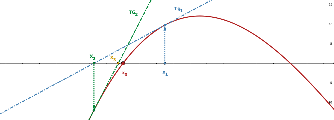
    Beim grafischen newtonschen Näherungsverfahren wird die Funktion durch eine Tangente Tg1 in einem geeignet gewählten Näherungswert x1 der tatsächlichen Nullstelle x0 ersetzt. Dort wo die Tangente Tg1 die x-Achse schneidet, wird erneut ein Näherungswert x2 bestimmt. Dabei liegt x2 schon viel näher an der tatsächlichen Nullstelle x0 als dies noch bei x1 der Fall war. Die nächste Näherung x3 wird mittels der Tangente Tg2 bestimmt. Dabei liegt x3 schon viel näher an der tatsächlichen Nullstelle x0 als dies noch bei x1 und x2 der Fall war....

    Bild
    Illustration newtonsches Näherungsverfahren

    Die Lösungen der Gleichung f(x)=0 stimmen mit den Nullstellen der Funktion f(x) überein. Im Intervall \(\left[ {{x_1};{x_2}} \right]\) befindet sich nur dann mindestens eine Nullstelle x0 der Funktion f(x), wenn f(x) dort stetig ist und f(x1) und f(x2) unterschiedliche Vorzeichen besitzen.

    Nullstelle einer Funktion
    Regula Falsi (Differenzierbarkeit)
    Sekantenverfahren (Differenzierbarkeit)
    Newtonsches Näherungsverfahren
    Fragen oder Feedback

    Schon den nächsten Urlaub geplant?
    Auf maths2mind kostenlos auf Prüfungen vorbereiten!
    Nach der Prüfung in Ruhe entspannen

    Startseite
    rgb(244,123,130)
    Bild
    Illustration Medidation 1050x450
    Startseite
    Wissenspfad
    Aufgaben

    Wichtige Funktionswerte im Zuge einer Kurvendiskussion

    Im Rahmen von Kurvendiskussionen untersucht man verschiedene Eigenschaften von Funktionen

    • Definitionsmenge, Stetigkeit und Differenzierbarkeit
    • Polstellen und Lücken
    • Verhalten im Unendlichen sowie Asymptotengleichungen
    • Symmetrie sowie Periodizität
    • Ableitungen f‘(x), f‘‘(x), f‘‘‘(x)
    • Nullstellen f(x)=0 sowie Schnittpunkt mit der y-Achse f(0)
    • Extremwerte (Hoch- und Tiefpunkte)
    • Wendepunkte und Sattelpunkte
    • Wendetangente
    • Krümmungsverhalten und Monotonie
    • Charakteristische Wertetabelle
    • Graph der Funktion mit Wendetangente(n)

    Extremstellen einer Funktion

    Unter den Extremstellen einer Funktion versteht man deren Minimum bzw. Maximum. Wenn eine Funktion in einem geschlossenen Intervall stetig ist, dann hat sie darin auch ein Minimum und ein Maximum.

    • notwendiges Kriterium: \(f'\left( x \right) = 0\)
    • hinreichendes Kriterium: \(f'' \ne 0\)
    • Minimum, wenn \(f'' > 0\)
    • Maximum, wenn \(f'' < 0\)

    Lokaler Extremwert

    Ein lokaler Extremwert liegt vor, wenn es keinen kleineren / größeren Funktionswert in der unmittelbaren Nähe am Funktionsgraph gibt.


    Absoluter bzw. globaler Extremwert

    Ein absoluter Extremwert ist der kleinste / größte von allen lokalen Extremwerten.


    Wendestelle einer Funktion

    Im Wendepunkt bzw. an der Wendestelle ändert sich das Krümmungsverhalten vom Graphen der Funktion. Eine Linkskrümmung geht in eine Rechtskrümmung bzw. umgekehrt über. Nur im Wendepunkt schneidet eine Tangente an den Graph der Funktion diesen Graph. Ein Wendepunkt mit horizontaler Wendetangente heißt Sattelpunkt

    An einer Wendestelle / im Wendepunkt gilt: \(f''\left( {{x_{WP}}} \right) = 0{\text{ sowie }}f'''\left( {{x_{WP}}} \right) \ne 0\)

    • Ein Polynom vom \({\text{Grad }} \geqslant 3\) muss mindestens eine Wendestelle haben.
    • Ein Polynom n-ten Grades kann maximal n-2 Wendestellen haben.

    Monotonie von Funktionen

    Steigt/fällt der Graph einer Funktion an jeder Stelle, so heißt die Funktion streng monoton steigend / fallend. Gibt es auch Stellen, an denen die Funktion weder steigt noch fällt, also konstant bleibt und daher parallel zur x-Achse verläuft, so fällt das Word „streng“ weg und die Funktion ist „nur“ monoton steigend / fallend. Aussagen betreffend Monotonie in bestimmten Intervalle der Funktion leitet man daraus ab, ob dort die ersten Ableitung \(f'\left( x \right)\) größer oder kleiner Null ist.

    \(\eqalign{ & \forall {x_1},{x_2} \in {D_f}{\text{ mit }}{x_1} < {x_2} \Rightarrow f\left( {{x_1}} \right) < f\left( {{x_2}} \right){\text{ streng monoton wachsend}} \cr & \forall {x_1},{x_2} \in {D_f}{\text{ mit }}{x_1} < {x_2} \Rightarrow f\left( {{x_1}} \right) \leqslant f\left( {{x_2}} \right){\text{ monoton wachsend}} \cr & \forall {x_1},{x_2} \in {D_f}{\text{ mit }}{x_1} < {x_2} \Rightarrow f\left( {{x_1}} \right) > f\left( {{x_2}} \right){\text{ streng monoton fallend}} \cr & \forall {x_1},{x_2} \in {D_f}{\text{ mit }}{x_1} < {x_2} \Rightarrow f\left( {{x_1}} \right) \geqslant f\left( {{x_2}} \right){\text{ monoton fallend}} \cr}\)


    Definitionslücke

    Unter einer Definitionslücke versteht man einzelne Punkte einer Funktion, die aus dem Definitionsbereich ausgeschlossen sind. (Nullstellen des Nenners)

    Dort ist die Funktion also nicht definiert. Entweder nähert sich der Graph dort einer senkrechten Asymptote an, dann liegt eine Polstelle vor, oder es liegt eine hebbare Definitionslücke vor. Eine hebbare Definitionslücke liegt dann vor, wenn die Vielfachheit der Nullstellen im Zähler größer oder gleich der Vielfachheit der Nullstellen im Nenner sind. Dann lässt sich die Nullstelle durch Kürzen entfernen.

    Funktion f f(x) = x (x² - 1) / (x - 1) Strecke g Strecke g: Strecke [B, A] Punkt A A = (1, 2) f\left( x \right) = \frac{{\left( {{x^2} - 1} \right) \cdot x}}{{x - 1}} = \frac{{\left( {x + 1} \right) \cdot \left( {x - 1} \right) \cdot x}}{{\left( {x - 1} \right)}} = \left( {x + 1} \right) \cdot x Text1 = "f\left( x \right) = \frac{{\left( {{x^2} - 1} \right) \cdot x}}{{x - 1}} = \frac{{\left( {x + 1} \right) \cdot \left( {x - 1} \right) \cdot x}}{{\left( {x - 1} \right)}} = \left( {x + 1} \right) \cdot x" f\left( x \right) = \frac{{\left( {{x^2} - 1} \right) \cdot x}}{{x - 1}} = \frac{{\left( {x + 1} \right) \cdot \left( {x - 1} \right) \cdot x}}{{\left( {x - 1} \right)}} = \left( {x + 1} \right) \cdot x Text1 = "f\left( x \right) = \frac{{\left( {{x^2} - 1} \right) \cdot x}}{{x - 1}} = \frac{{\left( {x + 1} \right) \cdot \left( {x - 1} \right) \cdot x}}{{\left( {x - 1} \right)}} = \left( {x + 1} \right) \cdot x" f\left( x \right) = \frac{{\left( {{x^2} - 1} \right) \cdot x}}{{x - 1}} = \frac{{\left( {x + 1} \right) \cdot \left( {x - 1} \right) \cdot x}}{{\left( {x - 1} \right)}} = \left( {x + 1} \right) \cdot x Text1 = "f\left( x \right) = \frac{{\left( {{x^2} - 1} \right) \cdot x}}{{x - 1}} = \frac{{\left( {x + 1} \right) \cdot \left( {x - 1} \right) \cdot x}}{{\left( {x - 1} \right)}} = \left( {x + 1} \right) \cdot x" f\left( x \right) = \frac{{\left( {{x^2} - 1} \right) \cdot x}}{{x - 1}} = \frac{{\left( {x + 1} \right) \cdot \left( {x - 1} \right) \cdot x}}{{\left( {x - 1} \right)}} = \left( {x + 1} \right) \cdot x Text1 = "f\left( x \right) = \frac{{\left( {{x^2} - 1} \right) \cdot x}}{{x - 1}} = \frac{{\left( {x + 1} \right) \cdot \left( {x - 1} \right) \cdot x}}{{\left( {x - 1} \right)}} = \left( {x + 1} \right) \cdot x" f\left( x \right) = \frac{{\left( {{x^2} - 1} \right) \cdot x}}{{x - 1}} = \frac{{\left( {x + 1} \right) \cdot \left( {x - 1} \right) \cdot x}}{{\left( {x - 1} \right)}} = \left( {x + 1} \right) \cdot x Text1 = "f\left( x \right) = \frac{{\left( {{x^2} - 1} \right) \cdot x}}{{x - 1}} = \frac{{\left( {x + 1} \right) \cdot \left( {x - 1} \right) \cdot x}}{{\left( {x - 1} \right)}} = \left( {x + 1} \right) \cdot x" f\left( x \right) = \frac{{\left( {{x^2} - 1} \right) \cdot x}}{{x - 1}} = \frac{{\left( {x + 1} \right) \cdot \left( {x - 1} \right) \cdot x}}{{\left( {x - 1} \right)}} = \left( {x + 1} \right) \cdot x Text1 = "f\left( x \right) = \frac{{\left( {{x^2} - 1} \right) \cdot x}}{{x - 1}} = \frac{{\left( {x + 1} \right) \cdot \left( {x - 1} \right) \cdot x}}{{\left( {x - 1} \right)}} = \left( {x + 1} \right) \cdot x" f\left( x \right) = \frac{{\left( {{x^2} - 1} \right) \cdot x}}{{x - 1}} = \frac{{\left( {x + 1} \right) \cdot \left( {x - 1} \right) \cdot x}}{{\left( {x - 1} \right)}} = \left( {x + 1} \right) \cdot x Text1 = "f\left( x \right) = \frac{{\left( {{x^2} - 1} \right) \cdot x}}{{x - 1}} = \frac{{\left( {x + 1} \right) \cdot \left( {x - 1} \right) \cdot x}}{{\left( {x - 1} \right)}} = \left( {x + 1} \right) \cdot x" f\left( x \right) = \frac{{\left( {{x^2} - 1} \right) \cdot x}}{{x - 1}} = \frac{{\left( {x + 1} \right) \cdot \left( {x - 1} \right) \cdot x}}{{\left( {x - 1} \right)}} = \left( {x + 1} \right) \cdot x Text1 = "f\left( x \right) = \frac{{\left( {{x^2} - 1} \right) \cdot x}}{{x - 1}} = \frac{{\left( {x + 1} \right) \cdot \left( {x - 1} \right) \cdot x}}{{\left( {x - 1} \right)}} = \left( {x + 1} \right) \cdot x" f\left( x \right) = \frac{{\left( {{x^2} - 1} \right) \cdot x}}{{x - 1}} = \frac{{\left( {x + 1} \right) \cdot \left( {x - 1} \right) \cdot x}}{{\left( {x - 1} \right)}} = \left( {x + 1} \right) \cdot x Text1 = "f\left( x \right) = \frac{{\left( {{x^2} - 1} \right) \cdot x}}{{x - 1}} = \frac{{\left( {x + 1} \right) \cdot \left( {x - 1} \right) \cdot x}}{{\left( {x - 1} \right)}} = \left( {x + 1} \right) \cdot x" f\left( x \right) = \frac{{\left( {{x^2} - 1} \right) \cdot x}}{{x - 1}} = \frac{{\left( {x + 1} \right) \cdot \left( {x - 1} \right) \cdot x}}{{\left( {x - 1} \right)}} = \left( {x + 1} \right) \cdot x Text1 = "f\left( x \right) = \frac{{\left( {{x^2} - 1} \right) \cdot x}}{{x - 1}} = \frac{{\left( {x + 1} \right) \cdot \left( {x - 1} \right) \cdot x}}{{\left( {x - 1} \right)}} = \left( {x + 1} \right) \cdot x" f\left( x \right) = \frac{{\left( {{x^2} - 1} \right) \cdot x}}{{x - 1}} = \frac{{\left( {x + 1} \right) \cdot \left( {x - 1} \right) \cdot x}}{{\left( {x - 1} \right)}} = \left( {x + 1} \right) \cdot x Text1 = "f\left( x \right) = \frac{{\left( {{x^2} - 1} \right) \cdot x}}{{x - 1}} = \frac{{\left( {x + 1} \right) \cdot \left( {x - 1} \right) \cdot x}}{{\left( {x - 1} \right)}} = \left( {x + 1} \right) \cdot x" f\left( x \right) = \frac{{\left( {{x^2} - 1} \right) \cdot x}}{{x - 1}} = \frac{{\left( {x + 1} \right) \cdot \left( {x - 1} \right) \cdot x}}{{\left( {x - 1} \right)}} = \left( {x + 1} \right) \cdot x Text1 = "f\left( x \right) = \frac{{\left( {{x^2} - 1} \right) \cdot x}}{{x - 1}} = \frac{{\left( {x + 1} \right) \cdot \left( {x - 1} \right) \cdot x}}{{\left( {x - 1} \right)}} = \left( {x + 1} \right) \cdot x" f\left( x \right) = \frac{{\left( {{x^2} - 1} \right) \cdot x}}{{x - 1}} = \frac{{\left( {x + 1} \right) \cdot \left( {x - 1} \right) \cdot x}}{{\left( {x - 1} \right)}} = \left( {x + 1} \right) \cdot x Text1 = "f\left( x \right) = \frac{{\left( {{x^2} - 1} \right) \cdot x}}{{x - 1}} = \frac{{\left( {x + 1} \right) \cdot \left( {x - 1} \right) \cdot x}}{{\left( {x - 1} \right)}} = \left( {x + 1} \right) \cdot x" f\left( x \right) = \frac{{\left( {{x^2} - 1} \right) \cdot x}}{{x - 1}} = \frac{{\left( {x + 1} \right) \cdot \left( {x - 1} \right) \cdot x}}{{\left( {x - 1} \right)}} = \left( {x + 1} \right) \cdot x Text1 = "f\left( x \right) = \frac{{\left( {{x^2} - 1} \right) \cdot x}}{{x - 1}} = \frac{{\left( {x + 1} \right) \cdot \left( {x - 1} \right) \cdot x}}{{\left( {x - 1} \right)}} = \left( {x + 1} \right) \cdot x" f\left( x \right) = \frac{{\left( {{x^2} - 1} \right) \cdot x}}{{x - 1}} = \frac{{\left( {x + 1} \right) \cdot \left( {x - 1} \right) \cdot x}}{{\left( {x - 1} \right)}} = \left( {x + 1} \right) \cdot x Text1 = "f\left( x \right) = \frac{{\left( {{x^2} - 1} \right) \cdot x}}{{x - 1}} = \frac{{\left( {x + 1} \right) \cdot \left( {x - 1} \right) \cdot x}}{{\left( {x - 1} \right)}} = \left( {x + 1} \right) \cdot x" f\left( x \right) = \frac{{\left( {{x^2} - 1} \right) \cdot x}}{{x - 1}} = \frac{{\left( {x + 1} \right) \cdot \left( {x - 1} \right) \cdot x}}{{\left( {x - 1} \right)}} = \left( {x + 1} \right) \cdot x Text1 = "f\left( x \right) = \frac{{\left( {{x^2} - 1} \right) \cdot x}}{{x - 1}} = \frac{{\left( {x + 1} \right) \cdot \left( {x - 1} \right) \cdot x}}{{\left( {x - 1} \right)}} = \left( {x + 1} \right) \cdot x" f\left( x \right) = \frac{{\left( {{x^2} - 1} \right) \cdot x}}{{x - 1}} = \frac{{\left( {x + 1} \right) \cdot \left( {x - 1} \right) \cdot x}}{{\left( {x - 1} \right)}} = \left( {x + 1} \right) \cdot x Text1 = "f\left( x \right) = \frac{{\left( {{x^2} - 1} \right) \cdot x}}{{x - 1}} = \frac{{\left( {x + 1} \right) \cdot \left( {x - 1} \right) \cdot x}}{{\left( {x - 1} \right)}} = \left( {x + 1} \right) \cdot x" f\left( x \right) = \frac{{\left( {{x^2} - 1} \right) \cdot x}}{{x - 1}} = \frac{{\left( {x + 1} \right) \cdot \left( {x - 1} \right) \cdot x}}{{\left( {x - 1} \right)}} = \left( {x + 1} \right) \cdot x Text1 = "f\left( x \right) = \frac{{\left( {{x^2} - 1} \right) \cdot x}}{{x - 1}} = \frac{{\left( {x + 1} \right) \cdot \left( {x - 1} \right) \cdot x}}{{\left( {x - 1} \right)}} = \left( {x + 1} \right) \cdot x" f\left( x \right) = \frac{{\left( {{x^2} - 1} \right) \cdot x}}{{x - 1}} = \frac{{\left( {x + 1} \right) \cdot \left( {x - 1} \right) \cdot x}}{{\left( {x - 1} \right)}} = \left( {x + 1} \right) \cdot x Text1 = "f\left( x \right) = \frac{{\left( {{x^2} - 1} \right) \cdot x}}{{x - 1}} = \frac{{\left( {x + 1} \right) \cdot \left( {x - 1} \right) \cdot x}}{{\left( {x - 1} \right)}} = \left( {x + 1} \right) \cdot x" f\left( x \right) = \frac{{\left( {{x^2} - 1} \right) \cdot x}}{{x - 1}} = \frac{{\left( {x + 1} \right) \cdot \left( {x - 1} \right) \cdot x}}{{\left( {x - 1} \right)}} = \left( {x + 1} \right) \cdot x Text1 = "f\left( x \right) = \frac{{\left( {{x^2} - 1} \right) \cdot x}}{{x - 1}} = \frac{{\left( {x + 1} \right) \cdot \left( {x - 1} \right) \cdot x}}{{\left( {x - 1} \right)}} = \left( {x + 1} \right) \cdot x" f\left( x \right) = \frac{{\left( {{x^2} - 1} \right) \cdot x}}{{x - 1}} = \frac{{\left( {x + 1} \right) \cdot \left( {x - 1} \right) \cdot x}}{{\left( {x - 1} \right)}} = \left( {x + 1} \right) \cdot x Text1 = "f\left( x \right) = \frac{{\left( {{x^2} - 1} \right) \cdot x}}{{x - 1}} = \frac{{\left( {x + 1} \right) \cdot \left( {x - 1} \right) \cdot x}}{{\left( {x - 1} \right)}} = \left( {x + 1} \right) \cdot x" f\left( x \right) = \frac{{\left( {{x^2} - 1} \right) \cdot x}}{{x - 1}} = \frac{{\left( {x + 1} \right) \cdot \left( {x - 1} \right) \cdot x}}{{\left( {x - 1} \right)}} = \left( {x + 1} \right) \cdot x Text1 = "f\left( x \right) = \frac{{\left( {{x^2} - 1} \right) \cdot x}}{{x - 1}} = \frac{{\left( {x + 1} \right) \cdot \left( {x - 1} \right) \cdot x}}{{\left( {x - 1} \right)}} = \left( {x + 1} \right) \cdot x" f\left( x \right) = \frac{{\left( {{x^2} - 1} \right) \cdot x}}{{x - 1}} = \frac{{\left( {x + 1} \right) \cdot \left( {x - 1} \right) \cdot x}}{{\left( {x - 1} \right)}} = \left( {x + 1} \right) \cdot x Text1 = "f\left( x \right) = \frac{{\left( {{x^2} - 1} \right) \cdot x}}{{x - 1}} = \frac{{\left( {x + 1} \right) \cdot \left( {x - 1} \right) \cdot x}}{{\left( {x - 1} \right)}} = \left( {x + 1} \right) \cdot x" f\left( x \right) = \frac{{\left( {{x^2} - 1} \right) \cdot x}}{{x - 1}} = \frac{{\left( {x + 1} \right) \cdot \left( {x - 1} \right) \cdot x}}{{\left( {x - 1} \right)}} = \left( {x + 1} \right) \cdot x Text1 = "f\left( x \right) = \frac{{\left( {{x^2} - 1} \right) \cdot x}}{{x - 1}} = \frac{{\left( {x + 1} \right) \cdot \left( {x - 1} \right) \cdot x}}{{\left( {x - 1} \right)}} = \left( {x + 1} \right) \cdot x" f\left( x \right) = \frac{{\left( {{x^2} - 1} \right) \cdot x}}{{x - 1}} = \frac{{\left( {x + 1} \right) \cdot \left( {x - 1} \right) \cdot x}}{{\left( {x - 1} \right)}} = \left( {x + 1} \right) \cdot x Text1 = "f\left( x \right) = \frac{{\left( {{x^2} - 1} \right) \cdot x}}{{x - 1}} = \frac{{\left( {x + 1} \right) \cdot \left( {x - 1} \right) \cdot x}}{{\left( {x - 1} \right)}} = \left( {x + 1} \right) \cdot x" f\left( x \right) = \frac{{\left( {{x^2} - 1} \right) \cdot x}}{{x - 1}} = \frac{{\left( {x + 1} \right) \cdot \left( {x - 1} \right) \cdot x}}{{\left( {x - 1} \right)}} = \left( {x + 1} \right) \cdot x Text1 = "f\left( x \right) = \frac{{\left( {{x^2} - 1} \right) \cdot x}}{{x - 1}} = \frac{{\left( {x + 1} \right) \cdot \left( {x - 1} \right) \cdot x}}{{\left( {x - 1} \right)}} = \left( {x + 1} \right) \cdot x" f\left( x \right) = \frac{{\left( {{x^2} - 1} \right) \cdot x}}{{x - 1}} = \frac{{\left( {x + 1} \right) \cdot \left( {x - 1} \right) \cdot x}}{{\left( {x - 1} \right)}} = \left( {x + 1} \right) \cdot x Text1 = "f\left( x \right) = \frac{{\left( {{x^2} - 1} \right) \cdot x}}{{x - 1}} = \frac{{\left( {x + 1} \right) \cdot \left( {x - 1} \right) \cdot x}}{{\left( {x - 1} \right)}} = \left( {x + 1} \right) \cdot x" f\left( x \right) = \frac{{\left( {{x^2} - 1} \right) \cdot x}}{{x - 1}} = \frac{{\left( {x + 1} \right) \cdot \left( {x - 1} \right) \cdot x}}{{\left( {x - 1} \right)}} = \left( {x + 1} \right) \cdot x Text1 = "f\left( x \right) = \frac{{\left( {{x^2} - 1} \right) \cdot x}}{{x - 1}} = \frac{{\left( {x + 1} \right) \cdot \left( {x - 1} \right) \cdot x}}{{\left( {x - 1} \right)}} = \left( {x + 1} \right) \cdot x" f\left( x \right) = \frac{{\left( {{x^2} - 1} \right) \cdot x}}{{x - 1}} = \frac{{\left( {x + 1} \right) \cdot \left( {x - 1} \right) \cdot x}}{{\left( {x - 1} \right)}} = \left( {x + 1} \right) \cdot x Text1 = "f\left( x \right) = \frac{{\left( {{x^2} - 1} \right) \cdot x}}{{x - 1}} = \frac{{\left( {x + 1} \right) \cdot \left( {x - 1} \right) \cdot x}}{{\left( {x - 1} \right)}} = \left( {x + 1} \right) \cdot x" f\left( x \right) = \frac{{\left( {{x^2} - 1} \right) \cdot x}}{{x - 1}} = \frac{{\left( {x + 1} \right) \cdot \left( {x - 1} \right) \cdot x}}{{\left( {x - 1} \right)}} = \left( {x + 1} \right) \cdot x Text1 = "f\left( x \right) = \frac{{\left( {{x^2} - 1} \right) \cdot x}}{{x - 1}} = \frac{{\left( {x + 1} \right) \cdot \left( {x - 1} \right) \cdot x}}{{\left( {x - 1} \right)}} = \left( {x + 1} \right) \cdot x" f\left( x \right) = \frac{{\left( {{x^2} - 1} \right) \cdot x}}{{x - 1}} = \frac{{\left( {x + 1} \right) \cdot \left( {x - 1} \right) \cdot x}}{{\left( {x - 1} \right)}} = \left( {x + 1} \right) \cdot x Text1 = "f\left( x \right) = \frac{{\left( {{x^2} - 1} \right) \cdot x}}{{x - 1}} = \frac{{\left( {x + 1} \right) \cdot \left( {x - 1} \right) \cdot x}}{{\left( {x - 1} \right)}} = \left( {x + 1} \right) \cdot x" f\left( x \right) = \frac{{\left( {{x^2} - 1} \right) \cdot x}}{{x - 1}} = \frac{{\left( {x + 1} \right) \cdot \left( {x - 1} \right) \cdot x}}{{\left( {x - 1} \right)}} = \left( {x + 1} \right) \cdot x Text1 = "f\left( x \right) = \frac{{\left( {{x^2} - 1} \right) \cdot x}}{{x - 1}} = \frac{{\left( {x + 1} \right) \cdot \left( {x - 1} \right) \cdot x}}{{\left( {x - 1} \right)}} = \left( {x + 1} \right) \cdot x" f\left( x \right) = \frac{{\left( {{x^2} - 1} \right) \cdot x}}{{x - 1}} = \frac{{\left( {x + 1} \right) \cdot \left( {x - 1} \right) \cdot x}}{{\left( {x - 1} \right)}} = \left( {x + 1} \right) \cdot x Text1 = "f\left( x \right) = \frac{{\left( {{x^2} - 1} \right) \cdot x}}{{x - 1}} = \frac{{\left( {x + 1} \right) \cdot \left( {x - 1} \right) \cdot x}}{{\left( {x - 1} \right)}} = \left( {x + 1} \right) \cdot x" f\left( x \right) = \frac{{\left( {{x^2} - 1} \right) \cdot x}}{{x - 1}} = \frac{{\left( {x + 1} \right) \cdot \left( {x - 1} \right) \cdot x}}{{\left( {x - 1} \right)}} = \left( {x + 1} \right) \cdot x Text1 = "f\left( x \right) = \frac{{\left( {{x^2} - 1} \right) \cdot x}}{{x - 1}} = \frac{{\left( {x + 1} \right) \cdot \left( {x - 1} \right) \cdot x}}{{\left( {x - 1} \right)}} = \left( {x + 1} \right) \cdot x" f\left( x \right) = \frac{{\left( {{x^2} - 1} \right) \cdot x}}{{x - 1}} = \frac{{\left( {x + 1} \right) \cdot \left( {x - 1} \right) \cdot x}}{{\left( {x - 1} \right)}} = \left( {x + 1} \right) \cdot x Text1 = "f\left( x \right) = \frac{{\left( {{x^2} - 1} \right) \cdot x}}{{x - 1}} = \frac{{\left( {x + 1} \right) \cdot \left( {x - 1} \right) \cdot x}}{{\left( {x - 1} \right)}} = \left( {x + 1} \right) \cdot x" f\left( x \right) = \frac{{\left( {{x^2} - 1} \right) \cdot x}}{{x - 1}} = \frac{{\left( {x + 1} \right) \cdot \left( {x - 1} \right) \cdot x}}{{\left( {x - 1} \right)}} = \left( {x + 1} \right) \cdot x Text1 = "f\left( x \right) = \frac{{\left( {{x^2} - 1} \right) \cdot x}}{{x - 1}} = \frac{{\left( {x + 1} \right) \cdot \left( {x - 1} \right) \cdot x}}{{\left( {x - 1} \right)}} = \left( {x + 1} \right) \cdot x" f\left( x \right) = \frac{{\left( {{x^2} - 1} \right) \cdot x}}{{x - 1}} = \frac{{\left( {x + 1} \right) \cdot \left( {x - 1} \right) \cdot x}}{{\left( {x - 1} \right)}} = \left( {x + 1} \right) \cdot x Text1 = "f\left( x \right) = \frac{{\left( {{x^2} - 1} \right) \cdot x}}{{x - 1}} = \frac{{\left( {x + 1} \right) \cdot \left( {x - 1} \right) \cdot x}}{{\left( {x - 1} \right)}} = \left( {x + 1} \right) \cdot x" f\left( x \right) = \frac{{\left( {{x^2} - 1} \right) \cdot x}}{{x - 1}} = \frac{{\left( {x + 1} \right) \cdot \left( {x - 1} \right) \cdot x}}{{\left( {x - 1} \right)}} = \left( {x + 1} \right) \cdot x Text1 = "f\left( x \right) = \frac{{\left( {{x^2} - 1} \right) \cdot x}}{{x - 1}} = \frac{{\left( {x + 1} \right) \cdot \left( {x - 1} \right) \cdot x}}{{\left( {x - 1} \right)}} = \left( {x + 1} \right) \cdot x" f\left( x \right) = \frac{{\left( {{x^2} - 1} \right) \cdot x}}{{x - 1}} = \frac{{\left( {x + 1} \right) \cdot \left( {x - 1} \right) \cdot x}}{{\left( {x - 1} \right)}} = \left( {x + 1} \right) \cdot x Text1 = "f\left( x \right) = \frac{{\left( {{x^2} - 1} \right) \cdot x}}{{x - 1}} = \frac{{\left( {x + 1} \right) \cdot \left( {x - 1} \right) \cdot x}}{{\left( {x - 1} \right)}} = \left( {x + 1} \right) \cdot x" f\left( x \right) = \frac{{\left( {{x^2} - 1} \right) \cdot x}}{{x - 1}} = \frac{{\left( {x + 1} \right) \cdot \left( {x - 1} \right) \cdot x}}{{\left( {x - 1} \right)}} = \left( {x + 1} \right) \cdot x Text1 = "f\left( x \right) = \frac{{\left( {{x^2} - 1} \right) \cdot x}}{{x - 1}} = \frac{{\left( {x + 1} \right) \cdot \left( {x - 1} \right) \cdot x}}{{\left( {x - 1} \right)}} = \left( {x + 1} \right) \cdot x" f\left( x \right) = \frac{{\left( {{x^2} - 1} \right) \cdot x}}{{x - 1}} = \frac{{\left( {x + 1} \right) \cdot \left( {x - 1} \right) \cdot x}}{{\left( {x - 1} \right)}} = \left( {x + 1} \right) \cdot x Text1 = "f\left( x \right) = \frac{{\left( {{x^2} - 1} \right) \cdot x}}{{x - 1}} = \frac{{\left( {x + 1} \right) \cdot \left( {x - 1} \right) \cdot x}}{{\left( {x - 1} \right)}} = \left( {x + 1} \right) \cdot x" f\left( x \right) = \frac{{\left( {{x^2} - 1} \right) \cdot x}}{{x - 1}} = \frac{{\left( {x + 1} \right) \cdot \left( {x - 1} \right) \cdot x}}{{\left( {x - 1} \right)}} = \left( {x + 1} \right) \cdot x Text1 = "f\left( x \right) = \frac{{\left( {{x^2} - 1} \right) \cdot x}}{{x - 1}} = \frac{{\left( {x + 1} \right) \cdot \left( {x - 1} \right) \cdot x}}{{\left( {x - 1} \right)}} = \left( {x + 1} \right) \cdot x" f\left( x \right) = \frac{{\left( {{x^2} - 1} \right) \cdot x}}{{x - 1}} = \frac{{\left( {x + 1} \right) \cdot \left( {x - 1} \right) \cdot x}}{{\left( {x - 1} \right)}} = \left( {x + 1} \right) \cdot x Text1 = "f\left( x \right) = \frac{{\left( {{x^2} - 1} \right) \cdot x}}{{x - 1}} = \frac{{\left( {x + 1} \right) \cdot \left( {x - 1} \right) \cdot x}}{{\left( {x - 1} \right)}} = \left( {x + 1} \right) \cdot x" f\left( x \right) = \frac{{\left( {{x^2} - 1} \right) \cdot x}}{{x - 1}} = \frac{{\left( {x + 1} \right) \cdot \left( {x - 1} \right) \cdot x}}{{\left( {x - 1} \right)}} = \left( {x + 1} \right) \cdot x Text1 = "f\left( x \right) = \frac{{\left( {{x^2} - 1} \right) \cdot x}}{{x - 1}} = \frac{{\left( {x + 1} \right) \cdot \left( {x - 1} \right) \cdot x}}{{\left( {x - 1} \right)}} = \left( {x + 1} \right) \cdot x" f\left( x \right) = \frac{{\left( {{x^2} - 1} \right) \cdot x}}{{x - 1}} = \frac{{\left( {x + 1} \right) \cdot \left( {x - 1} \right) \cdot x}}{{\left( {x - 1} \right)}} = \left( {x + 1} \right) \cdot x Text1 = "f\left( x \right) = \frac{{\left( {{x^2} - 1} \right) \cdot x}}{{x - 1}} = \frac{{\left( {x + 1} \right) \cdot \left( {x - 1} \right) \cdot x}}{{\left( {x - 1} \right)}} = \left( {x + 1} \right) \cdot x"

    Obige Illustration zeigt eine Funktion die an der Stelle x=1 nicht definiert ist und in deren Definitionsbereich somit an dieser Stelle eine Lücke vorliegt. Durch Kürzen kann man an der Stelle x=1 dem Definitionsbereich den Wert "2" zuordnen. Der Definitionsbereich ist somit \({D_f} = {\Bbb R}\), die Lücke ist geschlossen, man spricht von einer "hebbaren Definitionslücke"


    Polstelle

    Eine Polstelle ist eine Definitionslücke einer Funktion, an der sich die Funktionswerte asymptotisch einer senkrechten Geraden annähern, diese aber nie erreichen. Die gebrochenrationale Funktion \(f\left( x \right) = \dfrac{{p\left( x \right)}}{{q\left( x \right)}}\) besitzt an der Stelle x0 eine Polstelle, wenn gilt: \(p\left( {x = {x_0}} \right) \ne 0{\text{ und }}q\left( {x = {x_0}} \right) = 0\). Die Polstellen findet man, indem man die Nullstellen des Terms in Nenner bestimmt.

    • Bei Polstellen mit Vorzeichenwechsel strebt die Funktion auf einer Seite nach + Unendlich während sie auf der anderen Seite nach - Unendlich strebt.
    • Bei Polstellen ohne Vorzeichenwechsel streben beide Seiten entweder nach + oder nach - Unendlich

    Funktion g g(x) = 1 / x f(x) = \frac{1}{x} Text2 = "f(x) = \frac{1}{x}" f(x) = \frac{1}{x} Text2 = "f(x) = \frac{1}{x}" f(x) = \frac{1}{x} Text2 = "f(x) = \frac{1}{x}" f(x) = \frac{1}{x} Text2 = "f(x) = \frac{1}{x}" f(x) = \frac{1}{x} Text2 = "f(x) = \frac{1}{x}" f(x) = \frac{1}{x} Text2 = "f(x) = \frac{1}{x}" f(x) = \frac{1}{x} Text2 = "f(x) = \frac{1}{x}" f(x) = \frac{1}{x} Text2 = "f(x) = \frac{1}{x}"


    Obige Illustration zeigt den Graph der Funktion \(f\left( x \right) = \dfrac{1}{x}\)

    • mit der x-Achse und der y-Achse als Asymptote
    • der an der Stelle x=0 eine Polstelle mit Vorzeichenwechsel aufweist


    Links- bzw. rechtsseitiger Grenzwert

    An einer Polstelle mit Vorzeichenwechsel verhält sich der Graph der Funktion von links bzw. von rechts betrachtet unterschiedlich.

    • Der linksseitige Grenzwert ist jener Funktionswert f(x) den man erhält, wenn man sich einem bestimmten Funktionsargument x0, entlang vom Funktionsgraphen von links kommend annähert. 
    • Der rechtsseitige Grenzwert ist jener Funktionswert f(x) den man erhält, wenn man sich einem bestimmten Funktionsargument x0, entlang vom Funktionsgraphen von rechts kommend annähert. 
    • Ist die Funktion an der Stelle x0 stetig, dann stimmen der links- und der rechtsseitige Grenzwert überein. 


    • Aus dem Inneren des Definitionsbereichs betrachtet kann man daher einen linksseitigen und einen rechtsseitigen Grenzwert ermitteln.
      In GeoGebra gibt es dafür die Befehle

      • LinksseitigerGrenzwert (Funktion, Polstelle)
      • RechtsseitigerGrenzwert (Funktion, Polstelle)

    Asymptote

    Eine Asymptote ist eine Gerade, der sich der Graph einer Funktion unbegrenzt annähert, sie aber nie erreicht.

    Dabei unterscheidet man zwischen senkrechten, waagrechten und schiefen Asymptoten. Kurven, die sich dem Graph einer anderen Funktion zunehmend annähern, bezeichnet man als asymptotische Kurven.

    • Zählergrad = Höchste Potenz im Zähler einer Funktion
    • Nennergrad = Höchste Potenz im Nenner einer Funktion
       
    • Zählergrad < Nennergrad: die Funktion hat die x-Achse als Asymptote
    • Zählergrad = Nennergrad: die Asymptote verläuft horizontal
    • Zählergrad = Nennergrad + 1: die Asymptote verläuft schief
    • Zählergrad > Nennergrad+1: zu der Funktion gibt es eine asymptotische Kurve
       
    • Senkrechte (=vertikale) Asymptoten sind dort, wo sich die Polstellen (Definitionslücken) einer Funktion befinden und in deren Nähe die Funktionswerte gegen unendlich streben. Die senkrechten Asymptoten finden sich dort wo der Nenner Nullstellen hat, die aber keine Nullstellen vom Zähler sind.

    Funktion g g(x) = x² / (x² - 1) Funktion f f(x) = 1 Funktion f f(x) = 1 Gerade h Gerade h: Gerade durch B, A Gerade i Gerade i: Gerade durch D, C f\left( x \right) = \frac{{{x^2}}}{{{x^2} - 1}} Text2 = "f\left( x \right) = \frac{{{x^2}}}{{{x^2} - 1}}" f\left( x \right) = \frac{{{x^2}}}{{{x^2} - 1}} Text2 = "f\left( x \right) = \frac{{{x^2}}}{{{x^2} - 1}}" f\left( x \right) = \frac{{{x^2}}}{{{x^2} - 1}} Text2 = "f\left( x \right) = \frac{{{x^2}}}{{{x^2} - 1}}" f\left( x \right) = \frac{{{x^2}}}{{{x^2} - 1}} Text2 = "f\left( x \right) = \frac{{{x^2}}}{{{x^2} - 1}}" f\left( x \right) = \frac{{{x^2}}}{{{x^2} - 1}} Text2 = "f\left( x \right) = \frac{{{x^2}}}{{{x^2} - 1}}" f\left( x \right) = \frac{{{x^2}}}{{{x^2} - 1}} Text2 = "f\left( x \right) = \frac{{{x^2}}}{{{x^2} - 1}}" f\left( x \right) = \frac{{{x^2}}}{{{x^2} - 1}} Text2 = "f\left( x \right) = \frac{{{x^2}}}{{{x^2} - 1}}" f\left( x \right) = \frac{{{x^2}}}{{{x^2} - 1}} Text2 = "f\left( x \right) = \frac{{{x^2}}}{{{x^2} - 1}}" f\left( x \right) = \frac{{{x^2}}}{{{x^2} - 1}} Text2 = "f\left( x \right) = \frac{{{x^2}}}{{{x^2} - 1}}" f\left( x \right) = \frac{{{x^2}}}{{{x^2} - 1}} Text2 = "f\left( x \right) = \frac{{{x^2}}}{{{x^2} - 1}}" f\left( x \right) = \frac{{{x^2}}}{{{x^2} - 1}} Text2 = "f\left( x \right) = \frac{{{x^2}}}{{{x^2} - 1}}" f\left( x \right) = \frac{{{x^2}}}{{{x^2} - 1}} Text2 = "f\left( x \right) = \frac{{{x^2}}}{{{x^2} - 1}}" y=1 Text1 = "y=1" y=1 Text1 = "y=1" y=1 Text1 = "y=1" x=1 Text3 = "x=1" x=1 Text3 = "x=1" x=1 Text3 = "x=1" x=-1 Text4 = "x=-1" x=-1 Text4 = "x=-1" x=-1 Text4 = "x=-1" x=-1 Text4 = "x=-1"

    Bei obenstehender Funktion gilt: Zählergrad = 2 = Nennergrad und daher hat die Funktion \(f\left( x \right) = \dfrac{{{x^2}}}{{{x^2} - 1}}\) die horizontal verlaufende Asymptote y=1; An den Stellen x=-1 bzw. x=1 hat die Funktion zudem Polstellen mit Vorzeichenwechsel

    Extremstellen einer Funktion
    Lokales Minimum einer Funktion
    Lokales Maximum einer Funktion
    Globales Minimum einer Funktion
    Globales Maximum einer Funktion
    Wendepunkt einer Funktion
    Sattelpunkt einer Funktion
    Monotonie einer Folge
    Streng monoton wachsende Funktion
    Streng monoton fallende Funktion
    Monoton fallende Funktion
    Monoton wachsende Funktion
    Polstelle
    Polstelle mit Vorzeichenwechsel
    Polstelle ohne Vorzeichenwechsel
    Asymptote
    Zählergrad
    Nennergrad
    Definitionslücke
    hebbare Definitionslücke
    Linksseitiger Grenzwert
    GeoGebra LinksseitigerGrenzwert
    Rechtsseitiger Grenzwert
    GeoGebra RechtsseitigerGrenzwert
    Wendestelle einer Funktion
    Fragen oder Feedback
    Wissenspfad
    Aufgaben

    Gerade und ungerade Funktionen

    Abhängig vom Symmetrieverhalten unterscheidet man zwischen geraden und ungeraden Funktionen.


    Gerade Funktion

    Gerade Funktionen sind symmetrisch zur y-Achse. Spiegelt man die Funktionswerte mit positivem x um die y-Achse, so erhält man die Funktionswerte mit negativem x.

    \(f\left( x \right) = f\left( { - x} \right)\)

    Beispiele für gerade Funktionen:

    • die konstante Funktion \(f\left( x \right) = c\)
    • die Betragsfunktion \(f\left( x \right) = \left| x \right|\)
    • die Potenzfunktion \(f\left( x \right) = a \cdot {x^n}{\text{ mit }}a \ne 0{\text{ und n gerade}}\)
    • die Polynomfunktion \({\text{f}}\left( x \right) = {a_0} + {a_1} \cdot x + {a_2} \cdot {x^2} + ... + {a_n} \cdot {x^n}{\text{ mit }}{{\text{a}}_1},{a_3},{a_{ungerade}} = 0\)
    • die Kosinusfunktion \(f\left( x \right) = \cos \left( x \right)\)
    • die Sekansfunktion \(f\left( x \right) = \sec \left( x \right)\)

    Funktion f f(x) = x² Funktion g g(x) = x⁴ f(x)=x^2 Text1 = "f(x)=x^2" f(x)=x^2 Text1 = "f(x)=x^2" f(x)=x^2 Text1 = "f(x)=x^2" f(x)=x^2 Text1 = "f(x)=x^2" f(x)=x^2 Text1 = "f(x)=x^2" f(x)=x^2 Text1 = "f(x)=x^2" f(x)=x^2 Text1 = "f(x)=x^2" f(x)=x^4 Text2 = "f(x)=x^4" f(x)=x^4 Text2 = "f(x)=x^4" f(x)=x^4 Text2 = "f(x)=x^4" f(x)=x^4 Text2 = "f(x)=x^4" f(x)=x^4 Text2 = "f(x)=x^4" f(x)=x^4 Text2 = "f(x)=x^4" f(x)=x^4 Text2 = "f(x)=x^4"


    Ungerade Funktion

    Ungerade Funktionen sind symmetrisch zum Ursprung. Dreht man die Funktionswerte mit positivem x um 180° um den Ursprung, so erhält man die Funktionswerte mit negativem x.

    \(f\left( x \right) = - f\left( { - x} \right)\)

    Beispiele für ungerade Funktionen

    • die Vorzeichenfunktion \(f\left( x \right) = \operatorname{sgn} \left( x \right)\)
    • die identische Funktion \(f\left( x \right) = x\)
    • die Potenzfunktion \(f\left( x \right) = a \cdot {x^n}{\text{ mit }}a \ne 0{\text{ und n ungerade}}\)
    • die Polynomfunktion \({\text{f}}\left( x \right) = {a_0} + {a_1} \cdot x + {a_2} \cdot {x^2} + ... + {a_n} \cdot {x^n}{\text{ mit }}{{\text{a}}_0},{a_2},{a_{gerade}} = 0\)
    • die Sinusfunktion \(f\left( x \right) = \sin \left( x \right)\)
    • die Tangensfunktion \(f\left( x \right) = \tan \left( x \right)\)

    Funktion f f(x) = x³ Funktion g g(x) = x⁵ f(x)=x^3 Text1 = "f(x)=x^3" f(x)=x^3 Text1 = "f(x)=x^3" f(x)=x^3 Text1 = "f(x)=x^3" f(x)=x^3 Text1 = "f(x)=x^3" f(x)=x^3 Text1 = "f(x)=x^3" f(x)=x^3 Text1 = "f(x)=x^3" f(x)=x^3 Text1 = "f(x)=x^3" f(x)=x^5 Text2 = "f(x)=x^5" f(x)=x^5 Text2 = "f(x)=x^5" f(x)=x^5 Text2 = "f(x)=x^5" f(x)=x^5 Text2 = "f(x)=x^5" f(x)=x^5 Text2 = "f(x)=x^5" f(x)=x^5 Text2 = "f(x)=x^5" f(x)=x^5 Text2 = "f(x)=x^5"

    Gerade Funktion
    Ungerade Funktion
    Fragen oder Feedback
    Wissenspfad
    Aufgaben

    Parameterfunktionen

    Parameterfunktionen enthalten in ihren Funktionsgleichungen nicht nur die abhängige y-Variable und die unabhängige x-Variable, sondern auch einen oder mehrere Parameter (a, b, c, d). Durch die Variation dieser Parameter streckt, staucht oder verschiebt man den Graph der Funktion.


    Parameter einer Sinusfunktion

    Über Parameter kann die Form von Funktionen verändert werden.
    \(f\left( x \right) = a \cdot \sin \left( {b \cdot x + c} \right) + d\)

    • Der Faktor a bewirkt eine Streckung oder Stauchung der „Höhe“ - der sogenannten Amplitude.
    • Der Faktor b bewirkt eine Änderung der Periodendauer - dem Kehrwert der Frequenz - also einer Streckung oder Stauchung in Richtung der x-Achse
    • Der Summand c im Argument bewirkt eine Phasenverschiebung (Zeitpunkt des „Null-Durchgangs) in Richtung der x-Achse (=Parallelverschiebung in Richtung der x-Achse).
    • Der Summand d bewirkt eine Parallelverschiebung der Funktion in Richtung der y-Achse.


    Funktionsschar

    Eine Schar ist eine Anzahl von Funktionsgraphen, die jeweils aus einer gegebenen Funktionsgleichung mit veränderlichen Parametern hervorgehen.

    Parameter einer Funktion
    Parameter einer Sinusfunktion
    Funktionsschar
    Fragen oder Feedback
    Wissenspfad
    Aufgaben

    Bijektive, injektive und surjektive Funktionen

    Abhängig von der Zuordnung zwischen den Elementen der Definitions- und der Wertemenge unterscheidet man zwischen bijektiven, injektiven und surjektiven Funktionen.


    Bijektivität

    Bijektiv oder umkehrbar eindeutig ist eine Funktion f(x) dann, wenn nicht nur jedem Element x der Definitionsmenge Df eindeutig ein Element y der Wertemenge Wf zugeordnet wird, sondern wenn auch umgekehrt zu jedem Element y der Wertemenge Wf genau ein Element x der Definitionsmenge Df gehört. Umkehrbar eindeutige Funktionen heißen auch „ein-eindeutig“. Die Zuordnung von Wertepaaren ist also in beide Richtungen eindeutig, daher „umkehrbar“ eindeutig. Bijektive Funktionen sind daher sowohl injektiv als auch surjektiv. 

    Um zu zeigen, dass eine Funktion bijektiv ist und somit eine Umkehrfunktion besitzt, muss man zeigen, dass sie

    • entweder streng monoton steigend ist, dh man zeigt, dass f'(x)>0 ist
    • oder dass sie streng monoton fallend ist, dh man zeigt, dass f'(x)<0 ist.
       

    \(\eqalign{ & f\left( x \right) = y\,\,\,\,\, \Leftrightarrow \,\,\,\,\,{f^{ - 1}}\left( y \right) = x \cr & {f^{ - 1}} = {\text{Umkehrfunktion}} \cr}\)

    Ellipse c Ellipse c: Ellipse mit Brennpunkten E, F durch C Ellipse c Ellipse c: Ellipse mit Brennpunkten E, F durch C Ellipse c_1 Ellipse c_1: Ellipse mit Brennpunkten E_1, F_1 durch C_1 Ellipse c_1 Ellipse c_1: Ellipse mit Brennpunkten E_1, F_1 durch C_1 Ellipse c_1 Ellipse c_1: Ellipse mit Brennpunkten E_1, F_1 durch C_1 Ellipse c_2 Ellipse c_2: Ellipse mit Brennpunkten E_2, F_2 durch C_2 Ellipse c_2 Ellipse c_2: Ellipse mit Brennpunkten E_2, F_2 durch C_2 Ellipse c_3 Ellipse c_3: Ellipse mit Brennpunkten E_3, F_3 durch C_3 Ellipse c_3 Ellipse c_3: Ellipse mit Brennpunkten E_3, F_3 durch C_3 Vektor u Vektor u: Vektor[G, H] Vektor u Vektor u: Vektor[G, H] Vektor v Vektor v: Vektor[I, J] Vektor v Vektor v: Vektor[I, J] Vektor w Vektor w: Vektor[K, L] Vektor w Vektor w: Vektor[K, L] Vektor a Vektor a: Vektor[M, N] Vektor a Vektor a: Vektor[M, N] Vektor b Vektor b: Vektor[O, P] Vektor b Vektor b: Vektor[O, P] Vektor d Vektor d: Vektor[Q, R] Vektor d Vektor d: Vektor[Q, R] W_f Text2 = "W_f" W_f Text2 = "W_f" x_1 Text3 = "x_1" x_1 Text3 = "x_1" x_2 Text4 = "x_2" x_2 Text4 = "x_2" x_3 Text5 = "x_3" x_3 Text5 = "x_3" y_1 Text6 = "y_1" y_1 Text6 = "y_1" y_2 Text7 = "y_2" y_2 Text7 = "y_2" y_3 Text8 = "y_3" y_3 Text8 = "y_3" D_f Text1 = "D_f" D_f Text1 = "D_f" x_1 Text3_1 = "x_1" x_1 Text3_1 = "x_1" x_2 Text4_1 = "x_2" x_2 Text4_1 = "x_2" x_3 Text5_1 = "x_3" x_3 Text5_1 = "x_3" y_1 Text6_1 = "y_1" y_1 Text6_1 = "y_1" y_2 Text7_1 = "y_2" y_2 Text7_1 = "y_2" y_3 Text8_1 = "y_3" y_3 Text8_1 = "y_3" W_f Text2_1 = "W_f" W_f Text2_1 = "W_f" D_f Text1_1 = "D_f" D_f Text1_1 = "D_f"


    Illustration einer bijektiven Funktion

    Funktion f f(x) = x³ f(x)=x³ Text1 = “f(x)=x³”


    Umkehrfunktion

    Eine bijektive Funktion ist immer invertierbar, sie hat also eine Umkehrfunktion. Eine Funktion f besitzt genau dann eine Umkehrfunktion f-1, wenn sie streng monoton steigend oder streng monoton fallend ist. Der Graph der Umkehrfunktion f-1 geht durch Spiegelung vom Funktionsgraphen f um die 1. Mediane hervor.


    Reziproke Funktion

    Der Kehrwert einer Funktion wird als reziproke Funktion bezeichnet. Achtung: Die reziproke Funktion ist ungleich der Umkehrfunktion

    \(g\left( x \right) = \dfrac{1}{{f\left( x \right)}}\)


    Illustration einer Funktion und ihrer Umkehrfunktion

    Funktion f f(x) = x Funktion g g(x) = 2^x Funktion h h(x) = ln(x) f Text1 = "f" f^-^1 Text2 = "f^-^1" f^-^1 Text2 = "f^-^1" f^-^1 Text2 = "f^-^1" 1. Mediane Text3 = "1. Mediane"


    Injektivität

    Injektivität bedeutet, dass bei einer Funktion jedes Element der Wertemenge höchstens einmal als Funktionswert angenommen wird. Jedes Element der Wertemenge wird höchstens von einem (oder keinem) Pfeil aus der Definitionsmenge getroffen.

    Ellipse c Ellipse c: Ellipse mit Brennpunkten E, F durch C Ellipse c Ellipse c: Ellipse mit Brennpunkten E, F durch C Ellipse c_1 Ellipse c_1: Ellipse mit Brennpunkten E_1, F_1 durch C_1 Ellipse c_1 Ellipse c_1: Ellipse mit Brennpunkten E_1, F_1 durch C_1 Vektor u Vektor u: Vektor[G, H] Vektor u Vektor u: Vektor[G, H] Vektor v Vektor v: Vektor[I, J] Vektor v Vektor v: Vektor[I, J] Vektor w Vektor w: Vektor[K, L] Vektor w Vektor w: Vektor[K, L] W_f Text2 = "W_f" W_f Text2 = "W_f" x_1 Text3 = "x_1" x_1 Text3 = "x_1" x_2 Text4 = "x_2" x_2 Text4 = "x_2" x_3 Text5 = "x_3" x_3 Text5 = "x_3" y_1 Text6 = "y_1" y_1 Text6 = "y_1" y_2 Text7 = "y_2" y_2 Text7 = "y_2" y_3 Text8 = "y_3" y_3 Text8 = "y_3" D_f Text1 = "D_f" D_f Text1 = "D_f" y_4 Text9 = "y_4" y_4 Text9 = "y_4"


    Illustration einer injektiven, aber nicht surjektiven Funktion

    Funktion h h(x) = ℯ^x f(x)=e^x Text3 = “f(x)=e^x” f(x)=e^x Text3 = “f(x)=e^x” f(x)=e^x Text3 = “f(x)=e^x” f(x)=e^x Text3 = “f(x)=e^x” f(x)=e^x Text3 = “f(x)=e^x” f(x)=e^x Text3 = “f(x)=e^x” f(x)=e^x Text3 = “f(x)=e^x”


    Surjektivität

    Surjektivität bedeutet, dass bei einer Funktion jedes Element der Wertmenge mindestens einmal als Funktionswert angenommen wird. Jedes Element der Wertemenge wird mindestens von einem (oder mehreren) Pfeil(en) aus der Definitionsmenge getroffen.

    Ellipse c Ellipse c: Ellipse mit Brennpunkten E, F durch C Ellipse c Ellipse c: Ellipse mit Brennpunkten E, F durch C Ellipse c_1 Ellipse c_1: Ellipse mit Brennpunkten E_1, F_1 durch C_1 Ellipse c_1 Ellipse c_1: Ellipse mit Brennpunkten E_1, F_1 durch C_1 Vektor u Vektor u: Vektor[G, H] Vektor u Vektor u: Vektor[G, H] Vektor v Vektor v: Vektor[I, J] Vektor v Vektor v: Vektor[I, J] Vektor w Vektor w: Vektor[S, T] Vektor w Vektor w: Vektor[S, T] W_f Text2 = "W_f" W_f Text2 = "W_f" x_1 Text3 = "x_1" x_1 Text3 = "x_1" x_2 Text4 = "x_2" x_2 Text4 = "x_2" x_3 Text5 = "x_3" x_3 Text5 = "x_3" y_1 Text6 = "y_1" y_1 Text6 = "y_1" y_2 Text7 = "y_2" y_2 Text7 = "y_2" D_f Text1 = "D_f" D_f Text1 = "D_f"


    Illustration einer surjektiven, aber nicht injektiven Funktion

    Funktion g g(x) = x² f(x)=x² Text2 = “f(x)=x²”

    Umkehrbar eindeutige Funktionen
    Umkehrfunktion
    Bijektiv
    Injektiv
    Eineindeutige Funktionen
    surjektiv
    Reziproke Funktion
    Fragen oder Feedback

    Schon den nächsten Urlaub geplant?
    Auf maths2mind kostenlos auf Prüfungen vorbereiten!
    Nach der Prüfung in Ruhe entspannen

    Startseite
    rgb(244,123,130)
    Bild
    Illustration Medidation 1050x450
    Startseite
    Wissenspfad
    Aufgaben

    Zuordnungen

    Von einer Zuordnung spricht man, wenn ein Wert eindeutig einem anderen Wert zugeordnet wird. Ein Wert wird durch die Zuordungsvorschrift von einem anderen Wert abhängig.


    Darstellungsformen für Zuordnungen

    Zuordnungen können als Pfeile, als Wertetabellen, als Linien- oder Punktdiagramme in einem Koordinatensystem (auf der x-Achse der unabhängige Wert, auf der y-Achse der abhängige Wert) oder in Form einer mathematisch formulierten Zuordungsvorschrift (etwa als Funktion) abgebildet werden.


    Proportionale Zuordnung

    Von einer proportionalen, auch direkt proportionalen Zuordnung spricht man, der Quotient aus dem abhängigen und dem unabhängigen Wert konstant, also für alle Zahlenpaare gleich, ist.

    \(\dfrac{{{\text{y - Wert}}}}{{{\text{x - Wert}}}}{\text{ = konstant}}\)


    Direkter Proportionalitätsfaktor

    Ist der Quotient zweier Werte konstant, so sind die beiden Werte direkt proportional. Der direkte Proportionalitätsfaktor ist der Quotient aus dem abhängigen y- und dem unabhängigen x-Wert.

    \({\text{k = }}\dfrac{{{\text{y - Wert}}}}{{{\text{x - Wert}}}}\)

    • Die Zahlenpaare xi, yi sind quotientengleich. Umgekehrt formuliert heißt eine Zuordnung proportional, wenn sich jeder y-Wert durch Multiplikation vom x-Wert mit dem Proportionalitätsfaktor ergibt.
    • Proportionale Zuordnungen sind vom Typ "Je mehr, desto mehr".
    • Verdoppelt bzw. halbiert man den unabhängigen Wert so verdoppelt bzw. halbiert sich auch der abhängige Wert.
    • Der Graph einer proportionalen Zuordnung ist eine Gerade durch den Ursprung.

    Strahl f Strahl f: Strahl durch L, K Strahl g Strahl g: Strahl durch L, N Strahl h Strahl h: Strahl durch L, W Punkt E E = (0.25, 0.25) Punkt E E = (0.25, 0.25) Punkt F F = (0.5, 0.5) Punkt F F = (0.5, 0.5) Punkt G G = (1, 1) Punkt G G = (1, 1) Punkt H H = (2, 2) Punkt H H = (2, 2) Punkt I I = (3, 3) Punkt I I = (3, 3) Punkt J J = (4, 4) Punkt J J = (4, 4) Punkt K K = (5, 5) Punkt K K = (5, 5) Punkt L L = (0, 0) Punkt L L = (0, 0) Punkt M M = (1, 2) Punkt M M = (1, 2) Punkt N N = (2, 4) Punkt N N = (2, 4) Punkt O O = (3, 6) Punkt O O = (3, 6) Punkt P P = (4, 8) Punkt P P = (4, 8) Punkt Q Q = (5, 10) Punkt Q Q = (5, 10) Punkt R R = (1, 0.5) Punkt R R = (1, 0.5) Punkt S S = (2, 1) Punkt S S = (2, 1) Punkt T T = (3, 1.5) Punkt T T = (3, 1.5) Punkt U U = (4, 2) Punkt U U = (4, 2) Punkt V V = (5, 2.5) Punkt V V = (5, 2.5) Punkt W W = (6, 3) Punkt W W = (6, 3) k=1 Text1 = “k=1” k=2 Text2 = “k=2” k=0,5 Text3 = “k=0,5”

    Beispiel:
    Stückzahl und Kosten

    1 Wiener Schnitzel → 12 € Kosten
    2 Wiener Schnitzel → 24 € Kosten
    3 Wiener Schnitzel → 36 € Kosten

    Die Zuordnungsvorschrift besagt, dass ein Wiener Schnitzel 12 € kostet, und dass die n-fache Anzahl an Wiener Schnitzel den n-fachen Preis kosten. k=12


    Antiproportionale Zuordnung

    Von einer antiproportionalen, auch indirektproportionalen Zuordnung spricht man, wenn das Produkt aus dem abhängigen und dem unabhängigen Wert konstant, also für alle Zahlenpaare gleich ist

    \({\text{x - Wert}} \cdot {\text{y - Wert = konstant}}\)


    Indirekter Proportionalitätsfaktor

    Ist das Produkt zweier Werte konstant, so sind die beiden Werte indirekt proportional. Der indirekte Proportionalitätsfaktor ist das Produkt aus dem unabhängigen x und dem abhängigen y-Wert.

    \({\text{k = x - Wert}} \cdot {\text{y - Wert}}\)

    • Die Zahlenpaare xi, yi sind produktgleich. Umgekehrt formuliert heißt eine Zuordnung antiproportional, wenn sich jeder y-Wert durch Multiplikation vom 1/x-Wert (Kehrwert) mit dem Proportionalitätsfaktor ergibt.
    • Antiproportionale Zuordnungen sind vom Typ "Je mehr, desto weniger".
    • Verdoppelt bzw. halbiert man den unabhängigen Wert, so halbiert bzw. verdoppelt sich der abhängige Wert.
    • Der Graph einer antiproportionalen Zuordnung ist ein Hyperbelast, welcher von oben unendlich nach rechts unendlich verläuft.

    Funktion f f(x) = Wenn(x > 0, 4 * 1 / x) Punkt E E = (0.5, 8) Punkt E E = (0.5, 8) Punkt F F = (1, 4) Punkt F F = (1, 4) Punkt G G = (4, 1) Punkt G G = (4, 1) Punkt H H = (8, 0.5) Punkt H H = (8, 0.5) Punkt I I = (16, 0.25) Punkt I I = (16, 0.25) k=4 Text1 = “k=4”

    Beispiel:
    Arbeiter und Dauer der Baustelle

    1 Arbeiter → Dauer der Baustelle 12 Tage
    2 Arbeiter → Dauer der Baustelle 6 Tage
    3 Arbeiter → Dauer der Baustelle 4 Tage

    Die Zuordnungsvorschrift besagt, dass 1 Arbeiter 12 Tage benötigt und dass sich bei jedem weiteren Arbeiter die Baustellendauer halbiert. 0 Arbeiter werden jedoch nie fertig. k=12.

    Zuordnungen
    Proportionale Zuordnung
    Antiproportionale Zuordnung
    Proportionalitätsfaktor
    Fragen oder Feedback
    Wissenspfad

    Mathematisches Modell

    Ein mathematisches Modell beschreibt das Zusammenspiel von einzelnen Komponenten eines komplexen Systems (aus der Natur), mit den Mitteln der Mathematik.


    Zweck der Modellbildung (Regelungstechnik)

    Das Modell ist dabei eine vereinfachte Darstellung des komplexen Systems. Bei der Modellbildung darf nur soweit vereinfacht werden, solange das Modell das System hinreichend genau repräsentiert.


    Vorgehen bei der Modellbildung (Regelungstechnik)

    Bei der Modellbildung klärt man zunächst ab, welche Größen und welche Zusammenhänge zur Beschreibung des komplexen Originalsystems überhaupt relevant sind. Zur Abbildung in ein mathematisches Modell beschreibt man die Zusammenhänge zwischen den Zustandsgrößen durch Gleichungen


    Black Box (Regelungstechnik)

    Um vom komplexen System (aus der Natur) zu einem Modell zu kommen, betrachtet man das komplexe System wie eine Black Box. Eine Black Box ist ein Objekt, von dem zunächst nur das Verhalten über definierte äußere Schnittstellen bekannt ist. Man hat also kein Wissen darüber, wie das Innere der Black Box aufgebaut ist.

    Um ein Modell über das unbekannte Innere der Black Box und somit ein Modell für das komplexe System aufstellen zu können, verändert man gezielt den Input, also die Eingangsgrößen und beobachtet wie sich der Output, also die Ausgangsgrößen verändern und versucht dafür eine mathematische Funktion aufzustellen.

    Durch Parametervariation prüft man, ob die Ausgangsgrößen des realen komplexen Systems genauso den veränderten Parametern der Eingangsgrößen folgen, wie dies der Output der Black Box bei entsprechenden Veränderungen des Inputs macht.


    1. Schritt der Modellbildung

    Zunächst werden nur die Ein- bzw. Ausgangsgrößen untersucht:
    \(Input \to \boxed{BlackBox} \to Output\)


    2. Schritt der Modellbildung

    Dann wird versucht, die innere unbekannte Struktur zu modellieren:
    \({\text{unabhängige Größe}} \to \boxed{Modell} \to {\text{abhängige Größe}}\)

    Unabhängige Größe im Regelkreis

    Unter der unabhängigen Größe, auch Stellgröße, im Sinne der Regelungstechnik, verstehen wir den erwünschten Wert am Ausgang vom Regelkreis. Aus dem Sollwert und dem vom Regelkreis-Ausgang rückgeführten Istwert wird durch Vergleich die Regelwertabweichung gebildet, die dem Regler mit der Absicht zugeführt wird, Übereinstimmung zwischen der Stellgröße und dem Istwert der Regelgröße herzustellen.

    Abhängige Größe im Regelkreis

    Unter der abhängigen Größe, auch Regelgröße, im Sinne der Regelungstechnik, verstehen wir das Ausgangssignal vom Regelkreis.


    3. Schritt der Modellbildung

    Letztlich versucht man einen mathematischen Zusammenhang zwischen der Änderung der Ausgangsgröße in Abhängigkeit von einer Änderung der Eingangsgröße herzustellen.
    \(x \in {D_f} \to \boxed{y = f\left( x \right)} \to y \in {W_f}\)

    Dabei unterscheidet man zwischen diskreten und kontinuierlichen Modellen.


    Diskretes Modell (Ausdruck für Quantisierbarkeit)

    In diskreten Modellen ändert sich der Anfangswert um ein bestimmtes Quantum oder ein ganzzahliges Vielfaches davon. Dieses Quantum hat dabei einen bestimmten Mindestwert. Dieser Mindestwert kann nicht beliebig klein werden, sondern es handelt sich um eine bestimmte Menge oder eine bestimmte Anzahl. Einen Zwischenwert (etwa die Hälfte) von diesem Mindestwert gibt es nicht.

    t f(x)
    0 \({{y_0}}\)
    \({\Delta t}\) \({{y_1}}\)
    \({2\Delta t}\) \({{y_2}}\)

    Beispiele:

    • Geldmünzen: Die kleinste Einheit die man mit Bargeld bezahlen kann ist 1 Cent. Einen halben Cent als Zwischenwert gibt es (als Bargeld) nicht
    • Quantenphysik und das Standardmodell der Elementarteilchen sind Teilgebiete der Physik, die sich der Quantisierung widmen , dort gibt es Energie nur in bestimmten nicht weiter teilbaren Mengen

    Kontinuierliches Modell (Ausdruck für Kontinuität)

    In kontinuierlichen Modellen ändert sich der Anfangswert stetig. Änderungen (Zu- oder Abnahme) können beliebig klein sein. Zum Zeitpunkt t beträgt er yt = y(t). Differentialgleichungen eignen sich zur Beschreibung von kontinuierlichen Systemen.

    Beispiel:
    Die Gleichung einer Geraden. Für jedes (unabhängige) x gibt es ein (abhängiges) y=f(x).


    Simulation zur Überprüfung des Modells

    In der Simulation stellt man zuerst fest, wie sich die Ausgangsgrößen des Modells in Abhängigkeit von den Eingangsgrößen verhalten.​ Man analysiert das mathematische Modell hinsichtlich der Existenz und deren Eindeutigkeit von Lösungen. Im Falle von Abweichungen des Modellverhaltens während der Simulation vom Verhalten des realen komplexen Systems, sucht man nach Modellfehlern bzw. nach Datenfehlern.

    Mathematisches Modell
    Modellbildung
    Simulation
    Black Box
    Parametervariation (Black Box)
    Diskretes Modell
    Kontinuierliches Modell
    Abhängige Größe im Regelkreis
    Unabhängige Größe im Regelkreis
    Fragen oder Feedback
    Wissenspfad
    Aufgaben

    Wachstum

    Unter Wachstum versteht man den Anstieg einer Messgröße im Verlauf der Zeit.

    • Positivwachstum: Zunahme
    • Negativwachstum: Abnahme, Zerfall oder Schrumpfung
    • Nullwachstum: über den Zeitverlauf hinweg bleibt die Messgröße konstant

    Wir unterscheiden folgende Wachstumsmodelle

    • Lineare Wachstumsmodelle
    • Exponentielle Wachstumsmodelle
    • Beschränkte exponentielle Wachstumsmodelle
    • Logistische Wachstumsmodelle

    Lineare Wachstumsmodelle

    Bei linearen Wachstumsmodellen kommt t in der Gleichung, die das Übertragungsverhalten beschreibt, nur in der 1. Potenz vor. In gleichen Zeitschritten, erfolgen gleiche absolute Änderungen. Die Wachstumsrate ist konstant. Wir unterscheiden diskrete und kontinuierliche Modelle

    \(f\left( t \right) = kt + d\)

    d Anfangswert an der Stelle t=0
    k Wachstumswert

    Diskretes lineares Wachstumsmodell

    Beim diskreten linearen Wachstumsmodell bleibt die absolute Änderung pro Schritt konstant.

    \(\Delta {y_n} = {\text{k wobei: k}} \in {\Bbb R}\)

    • Rekursive Form: \({y_{n + 1}} = {y_n} + k\)
    • Explizite Form: \({y_n} = {y_0} + n \cdot k\)

    Kontinuierliches lineares Wachstumsmodell

    Beim kontinuierlichen linearen Wachstumsmodell ist die mittlere Änderungsrate konstant und unabhängig von jeweils aktuellen Wert.

    \(\eqalign{ & \dfrac{{\Delta y}}{{\Delta t}} = k{\text{ mit }}k \in {\Bbb R} \cr & y\left( t \right) = {y_0} + k \cdot t \cr}\)


    Exponentielle Wachstumsmodelle

    Bei exponentiellen Wachstumsmodellen (gemäß Exponentialfunktionen) kommt t in der Gleichung, die das Übertragungsverhalten beschreibt, als Exponent (Hochzahl) vor. In (absolut) gleichgroßen Zeitschritten t, erfolgen relative (=prozentual) gleichgroße Änderungen des Funktionswerts N(t). Charakteristisch ist die am Anfang langsame, dann zunehmend schneller werdende Zunahme, die letztlich explosionsartig schnell wird (Kettenprozesse). Unbegrenzt exponentielles Wachstum kann es in der Natur nicht geben. Wir unterscheiden diskrete und kontinuierliche Modelle

    • exponentielles Wachstum:
      \(N(t) = {N_0} \cdot {e^{\lambda \cdot t}} = {N_0} \cdot {b^t}{\text{ mit }}\lambda {\text{ = ln}}\left( b \right)\)
       
    • exponentielle Abnahme:
      \(N(t) = {N_0} \cdot {e^{ - \lambda \cdot t}}\)

    mit

    • N0 .. Startwert oder Anfangsbestand
    • b ... Wachstumsfaktor
    • \(\lambda > 0\)

    Diskretes exponentielles Wachstumsmodell

    Beim diskreten exponentiellen Wachstumsmodell ist die relative Änderung pro Schritt konstant. Die Wachstumsrate ist proportional zum Bestand.

    \(\dfrac{{\Delta {y_n}}}{{{y_n}}} = k{\text{ wobei: }}k \in {\Bbb R}\)

    • Rekursive Form: \({y_{n + 1}} = \left( {1 + k} \right) \cdot {y_n}\)
    • Explizite Form: \({y_n} = {y_0} \cdot {\left( {1 + k} \right)^n}\)

    Kontinuierlich exponentielles Wachstumsmodell

    Beim kontinuierlichen exponentiellen Wachstumsmodell ist die mittlere Änderungsrate proportional zum jeweils aktuellen Wert.

    \(\eqalign{ & \dfrac{{\Delta y}}{{\Delta t}} = k \cdot y\left( t \right){\text{ mit }}k \in {\Bbb R} \cr & y\left( t \right) = {y_0} \cdot {\left( {1 + k} \right)^t} \cr}\)


    Beschränkte exponentielle Wachstumsmodelle

    Bei beschränkten Wachstumsmodellen gibt es einen das Wachstum beschränkenden Wert S, wodurch das Wachstum nach oben oder nach unten beschränkt wird. Es handelt sich um ein sogenanntes Sättigungsmodell. Die absolute Änderung je Schritt ist proportional dem jeweils verbleibenden Abstand zur endlichen Obergrenze. Charakteristisch ist die Anfangs explosionsartig, dann zunehmend langsamer werdende Zunahme, die letztlich völlig abklingt und einer endlichen Obergrenze zustrebt. Wir unterscheiden diskrete und kontinuierliche Modelle

    • beschränktes exponentielles Wachstum:
      \(N\left( t \right) = S - a \cdot {e^{ - \lambda \cdot t}}\)
    • beschränktes exponentielle Abnahme:
      \(N\left( t \right) = S + a \cdot {e^{ - \lambda \cdot t}}\)

    mit:

    • S ... Sättigungswert
    • a=|S-N0|

    Kontinuierlich beschränktes Wachstumsmodell

    Beim kontinuierlich beschränkten Wachstumsmodell (z.B.: gemäß Logarithmusfunktionen) können bis zum Erreichen des Sättigungswertes alle Zwischenwerte auftreten

    \(f\left( x \right) = S - \left( {S - k} \right){e^{ - cx}}\)

    Als Maß für die Steigung dient die 1. Ableitung
    \(f'\left( x \right) = c \cdot \left( {S - f\left( x \right)} \right)\)

    wobei: k=f(0)

    Diskret beschränktes Wachstumsmodell

    Beim diskreten beschränkten Wachstumsmodell (z.B. Verkaufte Stückzahl von einem Produkt) können bis zum Erreichen des Sättigungswertes nur eine endliche Anzahl an diskreten Zwischenwerten auftreten.

    mit S als Sättigungswert:
    \(\Delta {y_n} = k \cdot \left( {S - {y_n}} \right)\)

    • Rekursive Form: \({y_{n + 1}} = {y_n} + k\left( {S - {y_n}} \right)\)
    • Explizite Form: \({y_n} = S - \left( {S - {y_0}} \right) \cdot {\left( {1 - k} \right)^n}\)

    Logistische Wachstumsmodelle

    Logistische Wachstumsmodelle sind eine Kombination aus exponentiellem und beschränktem Modell. Die absolute Änderung je Schritt ist proportional zum jeweiligen Wert N(t) und dem jeweils verbleibenden Abstand zur endlichen Obergrenze S.

    Kontinuierlich logistisches Wachstumsmodell

    Beim kontinuierlich logistischen Wachstumsmodell wächst der Bestand N(t) ausgehend von einem Startwert bzw. Anfangsbestand N0 zur Zeit t=0 zunächst exponentiell, wobei der s-förmige Graph dann einen Wendepunkt hat, ab dem sich das Wachstum abschwächst um sich einem Sättigungswert S anzunähern. Der Wendepunkt einer logistischen Wachstumsfunktion liegt immer beim halben Sättigungswert. Im Wendepunkt einer Funktion hat diese das größte Wachstum.

    \(N\left( t \right) = \dfrac{{{N_0} \cdot S}}{{{N_0} + \left( {S - {N_0}} \right) \cdot {e^{ - S \cdot k \cdot t}}}} = \dfrac{S}{{1 + \left( {\dfrac{S}{{{N_0}}} - 1} \right) \cdot {e^{ - S \cdot k \cdot t}}}} = \dfrac{S}{{1 + c \cdot {e^{ - \lambda \cdot t}}}}\)

    • N(t) ... Bestand zur Zeit t
    • N0 ... Anfangsbestand, Bestand zur Zeit t=0, Startwert N(0)
    • k ... Wachstumskonstante
    • S ... Sättigungswert, -schranke, -grenze

    Abbildung zur Veranschaulichung der Zusammenhänge bei logistischem Wachstum

    Bild
    Logistisches Wachstum

    Beispiel Grippe: Einige Touristen N0 bringen Grippeviren ins Land. Schnell infizieren sich immer mehr Menschen. Auf Grund von Immunisierung und dem Umstand dass die Wahrscheinlichkeit dass ein kranker Mensch einem noch gesunden Menschen begegnet mit Zunehmender Ausbreitung immer kleiner wird,  bremst sich der Zuwachs zunehmend ein, sodass am Ende der Epidemie eine bestimmte Anzahl der Bevölkerung S angesteckt ist. Die maximale Anzahl an Grippekranken ist natürlich mit 100% der Bevölkerung nach oben begrenzt.


    Diskretes logistisches Wachstumsmodell

    Beim diskreten logistischen Wachstumsmodell ist die absolute Änderung je Schritt proportional zum jeweiligen Wert und dem jeweils verbleibenden Abstand zur endlichen Obergrenze.

    \(\Delta {y_n} = k \cdot {y_n} \cdot \left( {S - {y_n}} \right)\)

    Rekursive Form:
    \({y_{n + 1}} = {y_n} + k \cdot {y_n} \cdot \left( {S - {y_n}} \right)\)

    Wachstum
    Positivwachstum
    Negativwachstum
    Nullwachstum
    Lineares Wachstum
    Beschränktes Wachstum
    Logistisches Wachstum
    Exponentielles Wachstum
    Beschränkte Abnahmemodelle
    Fragen oder Feedback

    Seitennummerierung

    • Aktuelle Seite 1
    • Page 2
    • Nächste Seite
    • Letzte Seite
    Aufgaben
    LösungswegBeat the Clock

    Aufgabe 110

    Eigenschaften von Funktionen

    Prüfe, ob eine Funktion vorliegt. Wähle alle richtigen Aussagen!

    Bild
    Bijektivität (Funktionen)


    • Aussage 1: Es liegt eine Funktion vor
    • Aussage 2: Es liegt keine Funktion vor
    • Aussage 3: Die vorliegende Funktion ist sogar bijektiv, injektiv und surjektiv
    Eigenschaften einer Funktion
    Bijektiv
    Injektiv
    surjektiv
    Fragen oder Feedback

    Schon den nächsten Urlaub geplant?
    Auf maths2mind kostenlos auf Prüfungen vorbereiten!
    Nach der Prüfung in Ruhe entspannen

    Startseite
    rgb(244,123,130)
    Bild
    Illustration Medidation 1050x450
    Startseite
    LösungswegBeat the Clock

    Aufgabe 111

    Eigenschaften von Funktionen

    Prüfe, ob eine Funktion vorliegt. Wähle alle richtigen Aussagen!

    Ellipse D_f Ellipse D_f: Ellipse mit Brennpunkten A, B durch C Ellipse D_f Ellipse D_f: Ellipse mit Brennpunkten A, B durch C Ellipse W_f Ellipse W_f: Ellipse mit Brennpunkten D, E durch F Ellipse W_f Ellipse W_f: Ellipse mit Brennpunkten D, E durch F Vektor u Vektor u: Vektor[x_4, y_1] Vektor u Vektor u: Vektor[x_4, y_1] Vektor v Vektor v: Vektor[x_1, y_2] Vektor v Vektor v: Vektor[x_1, y_2] Vektor w Vektor w: Vektor[x_3, y_4] Vektor w Vektor w: Vektor[x_3, y_4] D_f Text1 = "D_f" D_f Text1 = "D_f" W_f Text2 = "W_f" W_f Text2 = "W_f" x_1 Text3 = "x_1" x_1 Text3 = "x_1" x_2 Text4 = "x_2" x_2 Text4 = "x_2" x_3 Text5 = "x_3" x_3 Text5 = "x_3" y_1 Text6 = "y_1" y_1 Text6 = "y_1" y_2 Text7 = "y_2" y_2 Text7 = "y_2" y_3 Text8 = "y_3" y_3 Text8 = "y_3" x_4 Text3_1 = "x_4" x_4 Text3_1 = "x_4"

    • Aussage 1: Es liegt eine Funktion vor
    • Aussage 2: Es liegt keine Funktion vor
    • Aussage 3: Die vorliegende Funktion ist sogar bijektiv, injektiv und surjektiv
    Eigenschaften einer Funktion
    Bijektiv
    Injektiv
    surjektiv
    Fragen oder Feedback
    LösungswegBeat the Clock

    Aufgabe 112

    Eigenschaften von Funktionen

    Prüfe, ob eine Funktion vorliegt. Wähle alle richtigen Antworten!


    Bild
    Injektivität (Funktionen)


    • Aussage1 : Es liegt eine Funktion vor
    • Aussage 2: Es liegt keine Funktion vor
    • Aussage 3: Die vorliegende Funktion ist sogar injektiv, sie ist aber nicht surjektiv oder bijektiv.
    Eigenschaften einer Funktion
    Bijektiv
    Injektiv
    surjektiv
    Fragen oder Feedback
    LösungswegBeat the Clock

    Aufgabe 113

    Eigenschaften von Funktionen

    Prüfe, ob eine Funktion vorliegt. Wähle alle richtigen Antworten!

    Bild
    Eigenschaften einer Funktion


    • Aussage 1: Es liegt eine Funktion vor, die injektiv ist
    • Aussage 2: Es liegt keine Funktion vor
    • Aussage 3: Es liegt eine Funktion vor, die surjektiv ist
    • Aussage 4: Es liegt eine Funktion vor, die bijektiv ist
    • Aussage 5: Es liegt eine Funktion vor, die aber weder injektiv, noch surjektiv ist
    Eigenschaften einer Funktion
    Bijektiv
    Injektiv
    surjektiv
    Fragen oder Feedback
    LösungswegBeat the Clock

    Aufgabe 114

    Eigenschaften von Funktionen

    Prüfe, ob eine Funktion vorliegt. Wähle alle richtigen Antworten!

    Bild
    Eigenschaften einer Funktion


    • Aussage 1: Es liegt eine Funktion vor, die sogar surjektiv ist
    • Aussage 2: Es liegt keine Funktion vor, da x3 auf mehrere Elemente aus Wf verweist
    • Aussage 3: Es liegt keine Funktion vor, da auf y3 von den Elementen x2 und x3 aus Df verwiesen wird.
    • Aussage 4: Es liegt eine Funktion vor, die injektiv ist
    • Aussage 5: Es liegt eine Funktion vor
    Eigenschaften einer Funktion
    surjektiv
    Fragen oder Feedback

    Schon den nächsten Urlaub geplant?
    Auf maths2mind kostenlos auf Prüfungen vorbereiten!
    Nach der Prüfung in Ruhe entspannen

    Startseite
    rgb(244,123,130)
    Bild
    Illustration Medidation 1050x450
    Startseite
    LösungswegBeat the Clock

    Aufgabe 115

    Eigenschaften von Funktionen

    Prüfe, ob eine Funktion vorliegt. Wähle alle richtigen Antworten!

    Bild
    Eigenschaften einer Funktion


    • Aussage 1: Es liegt eine Funktion vor, die sogar surjektiv ist
    • Aussage 2: Es liegt keine Funktion vor, da x3 auf mehrere Elemente aus Wf verweist
    • Aussage 3: Es liegt keine Funktion vor, da auf y3 von den Elementen x2 und x3 aus Df verwiesen wird.
    • Aussage 4: Es liegt eine Funktion vor, die injektiv ist
    • Aussage 5: Es liegt eine Funktion vor
    Eigenschaften einer Funktion
    Bijektiv
    surjektiv
    Injektiv
    Fragen oder Feedback
    LösungswegBeat the Clock

    Aufgabe 116

    Eigenschaften von Funktionen

    Prüfe, ob eine Funktion \(f:{\Bbb R} \to {\Bbb R}\) vorliegt. Wähle alle richtigen Antworten!

    Bild
    Eigenschaften einer Funktion


    • Aussage 1: Es liegt eine Funktion vor
    • Aussage 2: Es liegt keine Funktion vor
    • Aussage 3: Es liegt eine Funktion vor, die sogar bijektiv ist
    Eigenschaften einer Funktion
    Bijektiv
    surjektiv
    Injektiv
    Fragen oder Feedback
    LösungswegBeat the Clock

    Aufgabe 117

    Eigenschaften von Funktionen

    Prüfe, ob eine Funktion \(f:{\Bbb R} \to {\Bbb R}\) vorliegt. Wähle alle richtigen Antworten!

    Bild
    Eigenschaften einer Funktion


    • Aussage 1: Es liegt keine Funktion vor
    • Aussage 2: Es liegt eine Funktion vor
    • Aussage 3: Es liegt eine Funktion vor, die sogar bijektiv ist
    Eigenschaften einer Funktion
    Bijektiv
    Fragen oder Feedback
    LösungswegBeat the Clock

    Aufgabe 118

    Eigenschaften von Funktionen

    Prüfe, ob eine Funktion \(f:{\Bbb R} \to {\Bbb R}\) vorliegt. Wähle alle richtigen Antworten!

    Funktion g g(x) = Wenn[(x > 0) ∧ (x < 2), x³ / 4, Wenn[x > 2, sin(x), x]] Strecke a Strecke a: Strecke [A, B]

    • Aussage 1: Es liegt eine Funktion vor
    • Aussage 2: Es liegt keine Funktion vor
    • Aussage 3: Es liegt eine Funktion vor, die sogar bijektiv ist
    Eigenschaften einer Funktion
    Bijektiv
    Fragen oder Feedback

    Schon den nächsten Urlaub geplant?
    Auf maths2mind kostenlos auf Prüfungen vorbereiten!
    Nach der Prüfung in Ruhe entspannen

    Startseite
    rgb(244,123,130)
    Bild
    Illustration Medidation 1050x450
    Startseite
    LösungswegBeat the Clock

    Aufgabe 119

    Eigenschaften von Funktionen

    Prüfe, ob eine Funktion \(f:{\Bbb R} \to {\Bbb R}\) vorliegt. Wähle alle richtigen Antworten!

    Bild
    Eigenschaften einer Funktion


    • Aussage 1: Es liegt keine Funktion vor
    • Aussage 2: Es liegt eine Funktion vor
    • Aussage 3: Es liegt eine Funktion vor. Die Funktion beschreibt einen Kreis, mit dem Mittelpunkt \(M({x_M}\left| {{y_M})} \right.\)
    Eigenschaften einer Funktion
    Fragen oder Feedback
    LösungswegBeat the Clock

    Aufgabe 120

    Eigenschaften von Funktionen

    Prüfe, ob eine Funktion \(f:{\Bbb R} \to {\Bbb R}\) vorliegt. Wähle alle richtigen Antworten!

    Bild
    Eigenschaften einer Funktion


    • Aussage 1: Es liegt keine Funktion vor.
    • Aussage 2: Es liegt eine Funktion vor.
    • Aussage 3: Es liegt eine Funktion vor. Die Funktion beschriebt die um 45° gedrehten Sinus-Funktion.
    Eigenschaften einer Funktion
    Fragen oder Feedback
    LösungswegBeat the Clock

    Aufgabe 121

    Eigenschaften von Funktionen

    Wähle alle richtigen Antworten!

    • Aussage 1: Es gibt Funktionen, die weder injektiv noch surjektiv sind
    • Aussage 2: Eine Funktion kann sowohl monoton steigende als auch monoton fallende Abschnitt beinhalten
    • Aussage 3: Jede Funktion muss entweder injektiv oder surjektiv oder bijektiv sein.
    • Aussage 4: Existiert eine Umkehrfunktion, dann ist die Funktion auch bijektiv
    Eigenschaften einer Funktion
    Injektiv
    surjektiv
    Bijektiv
    Monoton wachsende Funktion
    Monoton fallende Funktion
    Fragen oder Feedback

    Seitennummerierung

    • Aktuelle Seite 1
    • Page 2
    • Nächste Seite
    • Letzte Seite

    maths2mind®

    Kostenlos und ohne Anmeldung
    Lehrstoff und Aufgabenpool

    verständliche Erklärungen
    schneller Lernerfolg
    mehr Freizeit

    /
    Bild
    Illustration - Lady with Tablet
    /

    Maths2Mind ist ein einzigartiges Angebot, einerseits zur Mathematik-Matura bzw. Abiturvorbereitung, andererseits zur Vermittlung eines breiten Grundlagenwissens zu den MINT-Fächern Mathematik, Elektrotechnik und Physik, das sich von anderen Online-Ressourcen abhebt.

    Hier sind einige der wesentlichen Alleinstellungsmerkmale von maths2mind.com:

    • Kostenlose Prüfungsvorbereitung: Nicht jede Familie kann es sich leisten, für Prüfungsvorbereitung zu bezahlen. Nutzer von maths2mind benötigen keine Kreditkarte, da es keine kostenpflichtigen Abonnementpakete gibt. Alle Inhalte sind kostenlos zugänglich!
    • Privatsphäre: Es werden keine zustimmungspflichtigen Cookies verwendet, es gibt keine webseitenübergreifende oder personalisierte Werbung. 
    • Anonymes Lernen: Alle Inhalte sind ohne Anmeldung zugänglich, sodass Schüler anonym lernen können.
    • Autoren Dream-Team: Die Inhalte werden von Experten mit facheinschlägigem Universitätsabschluss erstellt. Zusätzlich erfolgte eine Recherche auf Vollständigkeit mittels künstlicher Intelligenz.
    • Probeschularbeiten: Lehrer können bei jeder Aufgabe einen Link kopieren, und durch simples "kopieren - einfügen" eine Probeschularbeit zusammenstellen und diese ihren Schülern elektronisch zum Selbststudium verfügbar machen.
    • Verständliche Erklärungen – schneller Lernerfolg – mehr Freizeit: Ehemalige Matura- bzw. Abiturbeispiele werden schriftlich vorgerechnet, damit Schüler den vollständigen Rechenweg 1:1 nachvollziehen können. Die ehemaligen Aufgaben sind sowohl chronologisch nach Prüfungstermin, als auch inhaltlich nach Lehrstoff sortiert, mittels anklickbarer Tags auffindbar.
    • Vernetzung von Lehrstoff und Rechenaufgaben über Tags: "Aufgaben passend zum Lernstoff" oder "Grundlagenwissen zur jeweiligen Aufgabe" sind mittels Tags leicht zu finden.
    • 1.000 Videos zum Rechenweg: Auch Dank der freundlichen Genehmigung des Bundesministeriums für Bildung, binden wir direkt in den Lösungsweg von Maturabeispielen, videobasierte Erklärungen ein.
    • 4.000 MINT-Fachbegriffe: Nutzer können gezielt nach Fachbegriffen suchen. Bei mehreren Treffern erfolgt die Auswahl über stichwortartige Zusammenfassungen.
    • 2.000 GeoGebra Illustrationen: Alle unsere rd. 2.000 selbst erstellten vektorbasierten Grafiken wurden mit GeoGebra erstellt. Zusätzlich verlinken wir auf anschauliche interaktive Illustrationen auf der GeoGebra Lernplattform.
    • Exzellent lesbare MINT-Inhalte: Die Inhalte sind vektorbasiert und daher auf allen Geräten, vom Smartphone bis zum XXL-Screen, gestochen scharf lesbar. Das gilt besonders für komplexe Formeln und anschauliche Illustrationen.
    • Wissenspfade: Zu jeder Lerneinheit werden gut strukturiert empfohlenes Vorwissen, verbreiterndes und vertiefendes Wissen angezeigt.
    • Umfassende Unterstützung: Maths2mind begleitet Schüler bis zum erfolgreichen Lehrabschluss mit Matura, dem Berufseinstieg nach Matura/Abitur und auch beim Studieneinstieg.
    • Soziale Mission: Als E-Learning Plattform mit sozialer Mission bietet maths2mind Chancen-Fairness durch genderneutralen Bildungszugang. Unabhängig von sozioökonomischem Umfeld, Wohnort, Einstellung oder Kulturkreis der Eltern, Sympathiewert des Lehrenden, finanzieller Schulausstattung oder Tagespolitik.
    • Kostenlose Fragen per E-Mail: Bei Unklarheiten können Fragen kostenlos per E-Mail gestellt werden.

    Maths2Mind.com ist somit eine umfassende Plattform, die nicht nur Wissen vermittelt, sondern auch auf individuelle Bedürfnisse eingeht und einen fairen Zugang zur Bildung ermöglicht.

    /

    Fußzeile

    • FAQ
    • Über maths2mind
    • Cookie Richtlinie
    • Datenschutz
    • Impressum
    • AGB
    • Blog

    © 2022 maths2mind GmbH